Page 199 - Computational Colour Science Using MATLAB

186 MULTISPECTRAL IMAGING

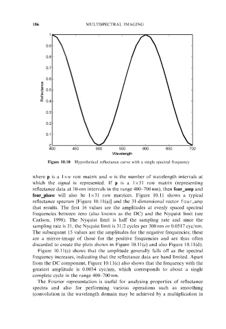
Figure 10.10 Hypothetical reflectance curve with a single spectral frequency

where p is a 1 w row matrix and w is the number of wavelength intervals at
which the signal is represented. If p is a 1 31 row matrix (representing
reflectance data at 10-nm intervals in the range 400–700 nm), then four_amp and
four_phase will also be 1 31 row matrices. Figure 10.11 shows a typical
reflectance specrum [Figure 10.11(a)] and the 31-dimensional vector four___amp
that results. The first 16 values are the amplitudes at evenly spaced spectral
frequencies between zero (also known as the DC) and the Nyquist limit (see
Carlson, 1998). The Nyquist limit is half the sampling rate and since the
sampling rate is 31, the Nyquist limit is 31/2 cycles per 300 nm or 0.0517 cyc/nm.
The subsequent 15 values are the amplitudes for the negative frequencies; these
are a mirror-image of those for the positive frequencies and are thus often
discarded to create the plots shown in Figure 10.11(c) and also Figure 10.11(d).
Figure 10.11(c) shows that the amplitude generally falls off as the spectral
frequency increases, indicating that the reflectance data are band limited. Apart
from the DC component, Figure 10.11(c) also shows that the frequency with the
greatest amplitude is 0.0034 cyc/nm, which corresponds to about a single
complete cycle in the range 400–700 nm.
The Fourier representation is useful for analysing properties of reflectance
spectra and also for performing various operations such as smoothing
(convolution in the wavelength domain may be achieved by a multiplication in