Page 58 - Computational Colour Science Using MATLAB

IMPLEMENTATIONS AND EXAMPLES 45

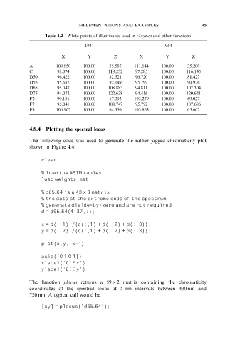
Table 4.2 White points of illuminants used in r2xyz.m and other functions
1931 1964

X Y Z X Y Z
A 109.850 100.00 35.585 111.144 100.00 35.200
C 98.074 100.00 118.232 97.285 100.00 116.145
D50 96.422 100.00 82.521 96.720 100.00 81.427
D55 95.682 100.00 92.149 95.799 100.00 90.926
D65 95.047 100.00 108.883 94.811 100.00 107.304
D75 94.072 100.00 122.638 94.416 100.00 120.641
F2 99.186 100.00 67.393 103.279 100.00 69.027
F7 95.041 100.00 108.747 95.792 100.00 107.686
F9 100.962 100.00 64.350 103.863 100.00 65.607

4.8.4 Plotting the spectral locus

The following code was used to generate the rather jagged chromaticity plot
shown in Figure 4.4:

clear

% load the ASTM tables
load weights.mat

% d65___64 is a 4363 matrix
% the data at the extreme ends of the spectrum
% generate divide-by-zero and are not required
d = d65___64(4:37,:);

x = d(:,1)./(d(:,1) + d(:,2) + d(:,3));
y = d(:,2)./(d(:,1) + d(:,2) + d(:,3));

plot(x,y,’k-’)

axis([0 1 0 1])
xlabel(’CIE x’)
ylabel(’CIE y’)

The function plocus returns a 5962 matrix containing the chromaticity
coordinates of the spectral locus at 5-nm intervals between 430 nm and
720 nm. A typical call would be

[xy] = plocus(’d65___64’);