Page 149 - Computational Fluid Dynamics for Engineers

Problems 135

(a) an explicit method and employing central differences for the boundary con-
ditions.
(b) an explicit method and employing forward differences for the boundary con-
ditions at x = 0
(c) the Crank-Nicolson method with central differences for the boundary con-
ditions.

Compare the numerical results obtained in each case with the analytical solution
given by
T(t, x) = e- an2t sin TT(X - 1/4)

Take a = 1, At = 0.0025 and Ax = 0.02.

4-8. Repeat Problem 4.6 with Keller's box method and compare your solutions
with those obtained in Problem 4.6.

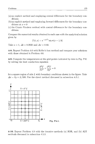
4-9. Compute the temperatures at the grid points indicated by dots in Fig. P41
by solving the heat conduction equation

2
2
d T d T _
dx 2 dy 2
for a square region of side L with boundary conditions shown in the figure. Take
Ax = 6y = L/100. Use the direct method discussed in subsection 4.5.1.

J V
A
T = 0°C
L

u
o
o u
i-H o
II
II
H
H

^
0 T = 2C )0°C > I W Fig. P4.1.

4-10. Repeat Problem 4.9 with the iterative methods (a) SOR, and (b) ADI
methods discussed in subsection 4.5.2.