Page 146 - Computational Fluid Dynamics for Engineers

132 4. Numerical Methods for Model Parabolic and Elliptic Equations

Example 4.7. Repeat Example 4.5 with the MV method by using two grids. Compare
your results with SOR, GS, ADI and MV for a convergence criterion of

max \Au — F\ < e = 0~ 7
=
1
Assume that h = Ax = Ay = 1/256.
=
SOR Gauss-Seidel ADI MV
h Iter MaxError Iter MaxError Iter MaxError Iter MaxError
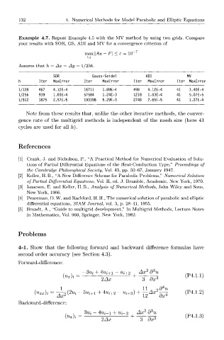
1/128 467 4.12E-4 16711 1.89E-4 498 4.12E-4 41 3.40E-4
1/256 939 1.03E-4 57584 1.24E-3 1218 1.03E-4 41 5.07E-5
1/512 1875 2.57E-5 193398 5.29E-3 2748 2.65E-5 41 1.27E-4

Note from these results that, unlike the other iterative methods, the conver-
gence rate of the multigrid methods is independent of the mesh size (here 41
cycles are used for all h).

References

[1] Crank, J. and Nicholson, P., "A Practical Method for Numerical Evaluation of Solu-
tions of Partial Differential Equations of the Heat-Conduction Type," Proceedings of
the Cambridge Philosophical Society, Vol. 43, pp. 50-67, January 1947.
[2] Keller, H. B., "A New Difference Scheme for Parabolic Problems," Numerical Solution
of Partial Differential Equations, Vol. II, ed. J. Bramble, Academic, New York, 1970.
[3] Isaacson, E. and Keller, H. B., Analysis of Numerical Methods, John Wiley and Sons,
New York, 1966.
[4] Peaceman, D. W. and Rachford, H. H., The numerical solution of parabolic and elliptic
differential equations, SI AM Journal, vol. 3, p. 28-41, 1955.
[5] Brandt, A., "Guide to multigrid development," In Multigrid Methods, Lecture Notes
in Mathematics, Vol. 960, Springer, New York, 1982.

Problems

4-1. Show that the following forward and backward difference formulas have
second order accuracy (see Section 4.3).
Forward-difference:

[Uxh + [ L
~ 2Ax 3 dx* '
1 11 d^u
3
{u xx)i = -^2 ( 2ui ~ 5 ^ + ! + 4ui + 2 ~ ^ + ) + \2 Ax2 ~dx^ (P4.1.2)
Backward-difference:

^ = 2Ax + ^ ~ d ^ ( P 4 ' 0 )