Page 141 - Computational Fluid Dynamics for Engineers

4.5 Finite-Difference Methods for Elliptic Equations 127

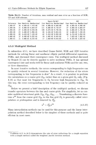
Table E 4 . l l . Number of iterations, max residual and max error as a function of SOR,
GS and ADI schemes.
SOR Gauss-Seidel ADI
Tolerance Iter MaxError MaxResidual Iter MaxError MaxResidual Iter MaxError MaxResidual
1.00E-07 36 6.68E-02 7.47E-08 154 6.68E-02 9.68E-08 19 6.68E-02 9.94E-08
1.00E-06 31 6.68E-02 6.62E-07 131 6.68E-02 9.73E-07 17 6.68E-02 6.82E-07
1.00E-05 27 6.68E-02 8.53E-06 108 6.67E-02 9.79E-06 15 6.68E-02 4.74E-06
1.00E-04 23 6.68E-02 5.98E-05 85 6.55E-02 9.85E-05 12 6.68E-02 7.15E-05
1.00E-03 20 6.63E-02 7.12E-04 62 5.31E-02 9.90E-04 10 6.71E-02 3.41E-04
1.00E-02 17 6.40E-02 9.30E-03 39 1.44E-01 9.94E-03 7 7.02E-02 7.56E-03
1.00E-01 11 3.98E-01 8.23E-02 17 1.66E+00 9.03E-02 5 9.32E-02 3.22E-02

4.5.3 Multigrid Method

In subsection 4.5.1, we have described Gauss-Seidel, SOR and ADI iterative
methods for solving linear and nonlinear elliptic partial differential equations,
PDEs, and discussed their convergence rates. The multigrid method discussed
by Brandt [5] can be directly applied to solve nonlinear PDEs. It has optimal
convergence rate and works well for linear and nonlinear PDEs and for one, two,
or three dimensions.
In most iterative methods, the errors corresponding to high frequencies can
be quickly reduced in several iterations. However, the reduction of the errors
corresponding to low frequencies is slow* As a result, it is prudent to perform
the calculations on a coarse grid f?2h rather than on a given grid j?^ only, (Fig.
4.10) so that most low frequencies in i?^ become high frequencies in 4?2/i- I n
this way, the error corresponding to low frequency can be quickly reduced on

Before we present a brief description of the multigrid method, we discuss
transfer operators between the fine and coarse grids. For simplicity, let us con-
sider multilevel structural grids i?2/i? ^4hi ^sh-, • • •• Transferring a discrete func-
tion u 2h from the coarse grid i? 2/i to the fine grid Q^ is generally called inter-
polation or prolongation and is denoted by J ^ .

u h = I% hu 2h (4.5.37)
Many interpolation methods can be used for this purpose and the linear inter-
polation method described below is the simplest of these methods and is quite
efficient in most cases.

* Problems 4-11 to 4-15 demonstrate the rate of error reductions for a simple equation
with a simple method called the weighted Jacobi iteration method.