Page 140 - Computational Fluid Dynamics for Engineers

126 4. Numerical Methods for Model Parabolic and Elliptic Equations

Column j
v//////^////,
* o + + known iterate (old value)
• o • o next iterate to be determined
+ + + + + o + + | | (newvalue)
Row / » o o o o o o o o * | o intermediate iterate
+ + + + + G + + I I • known value at boundary
• o +

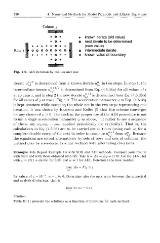
Fig. 4.9. ADI iteration by column and row.

iterate u™f is determined from a known iterate uf- in two steps. In step 1, the
intermediate iterate u™ • ' is determined from Eq. (4.5.36a) for all values of i
j
at column , and in step 2 the new iterate u^ 1 is determined from Eq. (4.5.36b)
for all values of j at row z, Fig. 4.9. The acceleration parameter UJ in Eqs. (4.5.36)
is kept constant while sweepinq the whole net in the two steps representing one
iteration. It was shown by Isaacson and Keller [3] that this scheme converges
for any choice of u > 0. The trick in the proper use of the ADI procedure is not
to use a single acceleration parameter UJ as above, but rather to use a sequence
of them, say u;i,u;2,.. ,cj m applied periodically (or cyclically). That is, the
•
calculations in Eq. (4.5.36) are to be carried out m times (using each uoi for a
complete double sweep of the net) in order to compute u™^ from n™ •. Because
the equations are solved alternatively by sets of rows and sets of columns, the
method may be considered as a line method with alternating directions.

Example 4.6. Repeat Example 4.5 with SOR and ADI methods. Compare your results
with SOR and with those obtained with GS. Take h = Ax = Ay = 1/10. Use Eq. (4.5.31a)
with u = 2/(1 + sin7r/i) for SOR and u = 1 for ADI. Determine the max residual

max \Au — F\2 < £
i,3
- n
for values of £ = 10 , n = 1 to 6. Determine also the max error between the numerical
and analytical solutions, that is
max|u,FDS — UAS\

Solution.
Table E4.ll presents the solutions as a function of iterations for each method.