Page 135 - Computational Fluid Dynamics for Engineers

4.5 Finite-Difference Methods for Elliptic Equations 121

can be used to solve Eq. (4.5.6). A listing of a subroutine for this purpose is
given in Table 4.3 for Aj, Bj and Cj matrices given by Eqs. (4.5.8a,b).
To use the subroutine in Table 4.3, the number of grid points in the x
J
and y directions must be specified by / (=11) and J (= J), respectively, the
coefficients 0 X (=TX), 6 y (=TY) in Eq. (4.5.4a), and the compound vector F
(=F) on the right-hand side of Eq (4.5.6). The compound vector F is obtained
from Eq (4.5.10) once the forcing function [/(#, y) in Eqs. (4.5.1)] is defined and
the boundary conditions on the four sides of the rectangle are given.

Example 4.5. Compute the temperature distribution in a square region of sides unity
subject to the following boundary conditions
T(x,0) = T ( x , l ) = 0, T(0,y) =smny and T(l,y) = e n sinny

by solving the heat condition equation,
2
2
d T d T
Compare your solutions with the analytical solution at x = 0.2, 0.5 and 0.9.
T(x, y) = e KX sin ny

Take Ax = Ay = 1/10.
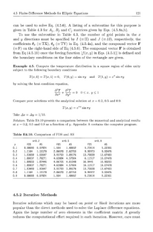
Solution. Table E4.10 presents a comparison between the numerical and analytical results
at x = 0.2, 0.5 and 0.9 as a function of y. Appendix A contains the computer program.

Table E4.10. Comparison of FDS and AS
x= 0.2 x= 0.5 X=l 0.9
y FDS AS FDS AS FDS AS
0.1 0.58693 0.57924 1.504 1.48652 5.23614 5.22301
0.2 1.1164 1.10178 2.86078 2.62753 9.95973 9.93476
0.3 1.53659 1.51647 3.93753 3.89176 13.70839 13.67403
0.4 1.80637 1.78271 4.62884 4.57504 6.11517 16.07478
0.5 1.89933 1.87446 4.86705 4.81048 16.9445 16.90203
0.6 1.80637 1.78271 4.62884 4.57504 16.11517 16.07478
0.7 1.53659 1.51647 3.93753 3.89176 13.70838 13.67403
0.8 1.1164 1.10178 2.86078 2.82753 9.95972 9.93476
0.9 0.58693 0.57924 1.504 1.48652 5.23614 5.22301

4.5.2 Iterative Methods

Iterative solutions which may be based on point or block iterations are more
popular than the direct methods used to solve the Laplace difference equations.
Again the large number of zero elements in the coefficient matrix A greatly
reduces the computational effort required in each iteration. However, care must