Page 130 - Computational Fluid Dynamics for Engineers

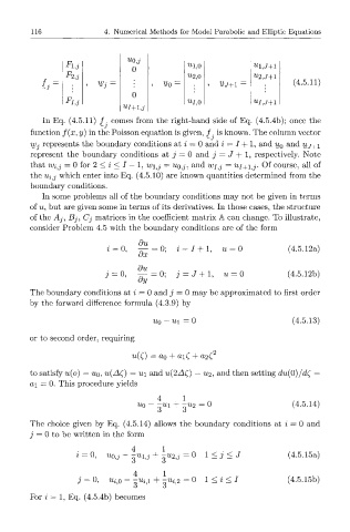
116 4. Numerical Methods for Model Parabolic and Elliptic Equations

u 0j
^1,0 U 1,J+1
0
F2J ^2,0 ^2,J+1
tj = WJ = % = ^ J + l (4.5.11)
0
FL: U/,0 U I,J+1
In Eq. (4.5.11) / . comes from the right-hand side of Eq. (4.5.4b); once the
~3
function f(x,y) in the Poisson equation is given, / . is known. The column vector
Wj represents the boundary conditions at i = 0 and i — I + 1, and u 0 and uj +i
represent the boundary conditions at j — 0 and j = J + 1, respectively. Note
that Wij = 0 for 2 < i < I — 1, w i j — IXOJ, and WJJ = UJ+IJ. Of course, all of
the ^j which enter into Eq. (4.5.10) are known quantities determined from the
i
boundary conditions.
In some problems all of the boundary conditions may not be given in terms
of u, but are given some in terms of its derivatives. In those cases, the structure
of the Aj, Bj, Cj matrices in the coefficient matrix A can change. To illustrate,
consider Problem 4.5 with the boundary conditions are of the form

du
0; i = J + l , u = 0 (4.5.12a)
dx
du
j = 0, ^ = 0 ; j = J + l, u = 0 (4.5.12b)
dy
The boundary conditions at i = 0 and j = 0 may be approximated to first order
by the forward difference formula (4.3.9) by

uo-ui =0 (4.5.13)
or to second order, requiring

u(C) = a 0 + ai( + a2( 2

to satisfy u(o) = UQ, U(AQ = u\ and u{2AQ — u 2l and then setting du(0)/d£ =
a\ = 0. This procedure yields
4 1 (4.5.14)
UQ - g^i + ^u 2 = 0
The choice given by Eq. (4.5.14) allows the boundary conditions at i — 0 and
j = 0 to be written in the form

i = 0, uoj -uij + -u 2j • 0 1 < j < J (4.5.15a)

4 1
j = 0, u ii0 - -Ui ti + -Uiz = 0 l<i<I (4.5.15b)
For i = 1, Eq. (4.5.4b) becomes