Page 128 - Computational Fluid Dynamics for Engineers

114 4. Numerical Methods for Model Parabolic and Elliptic Equations

XQ — 0, Xi = iAx, i = 1,2,... ,1,1+1 (4.5.2a)

2/o = 0, yj=jAy, j = 1,2,..., J, J + 1 (4.5.2b)
subject to the boundary conditions specified at four sides of the rectangle

i = (0,1 + 1) 0<j<J+l (4.5.3a)

j = (0, J + 1) 0 < i < I + 1 (4.5.3b)

n

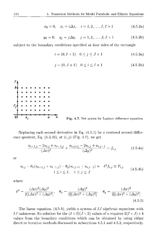
Fig. 4.7. Net points for Laplace difference equation.

Replacing each second derivative in Eq. (4.5.1) by a centered second differ-
ence quotient, Eq. (4.3.10), at (i,j) (Fig. 4.7), we get

+ / * xo — JiJ (4.5.4a)
(Ax) (Ay?
or

X
M
(4.5.4b)
l<i<I, l<j<J
where
(Axf(Ayf {Ayf (Ax)
6 2 = 2 2 x 2 v 2 2
2[(Ax) + (Ay) }' 2[(Ax)2 + (Ay) }' 2[(Ax) + (Ay) }

(4.5.5)
The linear equation, (4.5.4), yields a system of IJ algebraic equations with
2
IJ unknowns. Its solution for the (I + )(J + 2) values of u requires 2(1 + J) + 4
values from the boundary conditions which can be obtained by using either
direct or iterative methods discussed in subsections 4.5.1 and 4.5.2, respectively.