Page 124 - Computational Fluid Dynamics for Engineers

110 4. Numerical Methods for Model Parabolic and Elliptic Equations

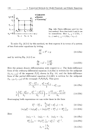
x a Unknown
x , = d A x Known
o "Centering"
T
h
x j - Vi t—t—i ,

*/-! Fig. 4.6. Finite-difference grid for the
-H/*i box method. Note that both h and k can
x 0=0. -» — t be nonuniform. Here t n_i = l/2(t n +
t n _ i ^, _ i/ 2 /„ £ n -i) and ^ _ i = 1/2(XJ +Xj-i).

To solve Eq. (4.2.4) by this method, we first express it in terms of a system
of two first-order equations by letting

T'=p (4.4.22a)
dx
and by writing Eq. (4.2.4) as

dp , ldT
(4.4.22b)
dx a ot
Here the primes denote differentiation with respect to x. The finite-difference
form of the ordinary differential equation (4.4.22a) is written for the midpoint
(£71,2^-1/2) °f the segment P1P2 shown in Fig. 4.6, and the finite-difference
form of the partial differential equation (4.4.22b) is written for the midpoint
x
(t"n-i/2-> j-i/2) of the rectangle P1P2P3P4' This gives

1 i +
j .7'-l Pj ^.7'-l
- Pj-l/2> (4.4.23a)
hj
_ n— 1
1 l P i / o - 1 !
P.i P.i-1 , Pi Pj-l
+ (4.4.23b)
hi a ^n
Rearranging both expressions we can write them in the form

Tn_ Tn_ x_h {pn +pn_ i)=^ (4.4.24a)

( Sl) jP? + {s 2) jPU + (ss)^ + Tf_ x) = Rp l/2. (4.4.24b)

Here
(s 2)j = - 1 , (33)j = -A. (4.4.25a)

J l
-"7-1/2 _ Z A J j-l/2 + ' P j - l ^ ' (4.4.25b)
7-I/2
rj-
lhj
= (4.4.25c)
ak„