Page 126 - Computational Fluid Dynamics for Engineers

112 4. Numerical Methods for Model Parabolic and Elliptic Equations

J
6 j = (4.4.31a)
iPjl
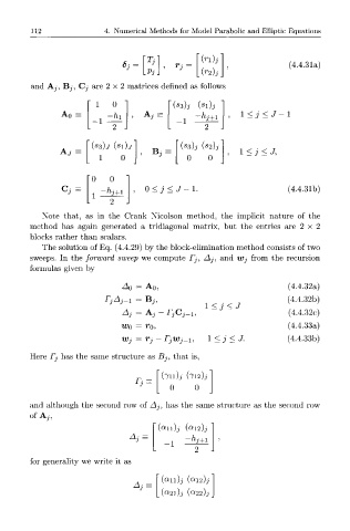
and Aj, B j , Cj are 2 x 2 matrices defined as follows

1 0 (*3)j ( S l ) j
An = , -hi A , = -h •j+i l<j<J-l
-1

(83)J (Sl)j (S3)j (82)j
A , = l<j<J,
1 0 0 0

0 0
Cj = -hj+i 0 < j < J - 1. (4.4.31b)
1

Note that, as in the Crank-Nicolson method, the implicit nature of the
method has again generated a tridiagonal matrix, but the entries are 2 x 2
blocks rather than scalars.
The solution of Eq. (4.4.29) by the block-elimination method consists of two
sweeps. In the forward sweep we compute Tj, Aj, and Wj from the recursion
formulas given by

AQ = A 0 , (4.4.32a)
rjAj-i Bj, (4.4.32b)
l<j<J
A3 = Aj r,-c (4.4.32c)
jV?'-i>
= r 0 , (4.4.33a)
w 0
r r w
Wj j~ j j-u 1<3<J. (4.4.33b)
Here fj has the same structure as Bj, that is,

(711 )j (712 )j
r,- 0 0

and although the second row of Aj, has the same structure as the second row
of A
3>
(a n)j (ai 2)j
{ h
3 = ~ J+i
1
2
for generality we write it as

["(an)j (ai 2)j
do =
-\7
[(<*2l)j («22)j