Page 123 - Computational Fluid Dynamics for Engineers

4.4 Finite-Difference Methods for Parabolic Equations 109

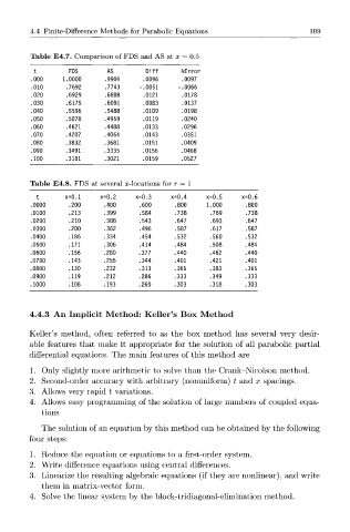
Table E4.7. Comparison of FDS and AS at x = 0.5

<-+ FDS AS Diff %Error
.000 1.0000 .9904 .0096 .0097
.010 .7692 .7743 -.0051 -.0066
.020 .6929 .6808 .0121 .0178
.030 .6175 .6091 .0083 .0137
.040 .5596 .5488 .0109 .0198
.050 .5078 .4959 .0119 .0240
.060 .4621 .4488 .0133 .0296
.070 .4207 .4064 .0143 .0351
.080 .3832 .3681 .0151 .0409
.090 .3491 .3335 .0156 .0468
.100 .3181 .3021 .0159 .0527

Table E4.8. FDS at several x-locations for r = 1
t x=0.1 x=0.2 x=0.3 x=0.4 x=0.5 x=0.6
.0000 .200 .400 .600 .800 1.000 .800
.0100 .213 .399 .584 .738 .769 .738
.0200 .210 .388 .543 .647 .693 .647
.0300 .200 .362 .496 .587 .617 .587
.0400 .186 .334 .454 .532 .560 .532
.0500 .171 .306 .414 .484 .508 .484
.0600 .156 .280 .377 .440 .462 .440
.0700 .143 .255 .344 .401 .421 .401
.0800 .130 .232 .313 .365 .383 .365
.0900 .119 .212 .286 .333 .349 .333
.1000 .108 .193 .260 .303 .318 .303

4.4.3 An Implicit Method: Keller's Box Method

Keller's method, often referred to as the box method has several very desir-
able features that make it appropriate for the solution of all parabolic partial
differential equations. The main features of this method are

1. Only slightly more arithmetic to solve than the Crank-Nicolson method.
2. Second-order accuracy with arbitrary (nonuniform) t and x spacings.
3. Allows very rapid t variations.
4. Allows easy programming of the solution of large numbers of coupled equa-
tions

The solution of an equation by this method can be obtained by the following
four steps:

1. Reduce the equation or equations to a first-order system.
2. Write difference equations using central differences.
3. Linearize the resulting algebraic equations (if they are nonlinear), and write
them in matrix-vector form.
4. Solve the linear system by the block-tridiagonal-elimination method.