Page 127 - Computational Fluid Dynamics for Engineers

4.5 Finite-Difference Methods for Elliptic Equations 113

In the backward sweep, 6j is computed from the following recursion formulas:

AJ6J = wj, (4.4.34a)
Aj6j = Wj - CjSj+u j = J - 1, J - 2 , . . . , 0. (4.4.34b)

Example 4.4. Repeat Example 4.1 using Keller's box method. Compare your results with
those obtained with the Crank-Nicolson method.

Solution. The solution of Example 4.4 with Keller's box method follows the procedure
described in subsection 4.4.3. Essentially after generating the finite-difference grid, initial
profiles at x = 0, we define (si)j to (ss)j in Eq. (4.4.25a) together with {r\)j and (r2)j.
Then we use SOLV2 to solve the linear system. Note that in this case wall and edge
temperatures are specified.
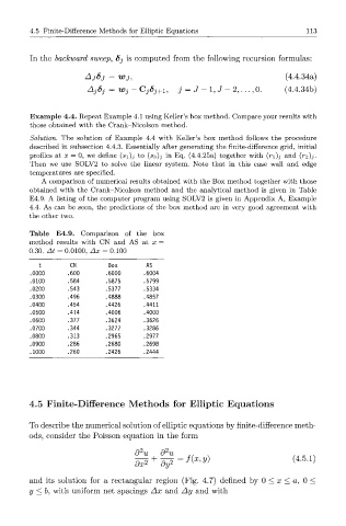
A comparison of numerical results obtained with the Box method together with those
obtained with the Crank-Nicolson method and the analytical method is given in Table
E4.9. A listing of the computer program using SOLV2 is given in Appendix A, Example
4.4. As can be seen, the predictions of the box method are in very good agreement with
the other two.

Table E4.9. Comparison of the box
method results with CN and AS at x =
0.30. At = 0.0100, Ax = 0.100

t CN Box AS
.0000 .600 .6000 .6004
.0100 .584 .5875 .5799
.0200 .543 .5377 .5334
.0300 .496 .4888 .4857
.0400 .454 .4426 .4411
.0500 .414 .4006 .4000
.0600 .377 .3624 .3626
.0700 .344 .3277 .3286
.0800 .313 .2965 .2977
.0900 .286 .2680 .2698
.1000 .260 .2426 .2444

4.5 Finite-Difference Methods for Elliptic Equations

To describe the numerical solution of elliptic equations by finite-difference meth-
ods, consider the Poisson equation in the form
2
2
d u d u

and its solution for a rectangular region (Fig. 4.7) defined by 0 < x < a, 0 <
y < b, with uniform net spacings Ax and Ay and with