Page 125 - Computational Fluid Dynamics for Engineers

4.4 Finite-Difference Methods for Parabolic Equations 111

Equations (4.4.24) are imposed for j = 1, , . . . , J — 1. At j = 0 and J, we
2
have
T 0 = T W, Tj = T e, (4.4.26)
respectively.
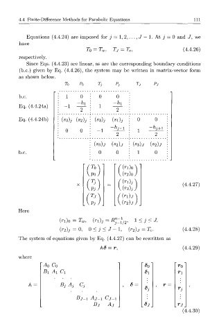
Since Eqs. (4.4.23) are linear, as are the corresponding boundary conditions
(b.c.) given by Eq. (4.4.26), the system may be written in matrix-vector form
as shown below.
To Po Tj Pi Tj Pj

b.c. : 1 0 '• 0 0
-hi -hi
Eq. (4.4.24a) : - 1 1
2 2
s
Eq. (4.4.24b) : ( s)j ( 2)j ( z)j (*i)i 0 0 :
s
s
-h j+i - / i j + i :
: 0 0 - 1 1
2 2 :
{sz)j {S2)j 0»3)j (« 2 )J 1
b.c. 0 0 1 0 :

To (n)o
Po (»*2)o
Tj (n)i
(4.4.27)
Pj
Tj f(n)j
Pj V(r 2)j
Here

(ri)o = T w, (ri)j = R]:l /2, 1 < j < J,
(r 2 ), = 0 , 0 < j < J - l , (r 2 )j = T e . (4.4.28)
The system of equations given by Eq. (4.4.27) can be rewritten as

= T\ (4.4.29)
where
A 0Co r^oi ~ r 0 l
Bi A x Ci Si n

Bj Aj Cj , 6 = , r =
*j r j
Bj-i Aj-i Cj-i
Bj Aj J . J. _rj\
6
(4.4.30)