Page 122 - Computational Fluid Dynamics for Engineers

108 4. Numerical Methods for Model Parabolic and Elliptic Equations

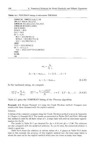
Table 4.1. FORTRAN listing of subroutine THOMAS.

SUBROUTINE THOMAS(II,A,B,C,T,R)
IMPLICIT REAL*8 (A-H,0-Z)
DIMENSION A(1),B(1),C(1),T(1),R(1)
DIMENSION BETA(201),S(201)
REAL*8 M(201)
BETA(l) = B(l)
S(l) = R(l)
DO I = 2,11
M(I) = A(I)/BETA(I-1)
BETA(I) = B(I)-M(I)*C(I-1)
S(I) = R(I)-M(I)*S(I-1)
ENDDO
T(II) = S(II)/BETA(II)
DO I = 11-1,1,-1
T(I) = (S(I)-C(I)*T(I+1))/BETA(I)
ENDDO
RETURN
END

mi = ^—
Pi-\

fa = bi -rriiCi-i, i = 2 , 3 , . . . , / - 1

Si = n - rrtiSi-i (4.4.20)
In the backward sweep, we compute

n l
o. _ rT +
T?^ = ^ - , T?+ l = ' p +1 , i = / - 2 , J - 3 , . . . , l (4.4.21)
PI-I Pi

Table 4.1 gives the FORTRAN listing of the Thomas algorithm.

Example 4.3. Repeat Example 4.1 using the Crank-Nicolson method. Compare your
results with these obtained with the explicit method.
Solution.
A listing of the computer program using the Crank-Nicolson method is given in Appendix
A, Chapter 4, Example E4.3. The results are presented in Tables E4.7 and E4.8. Although
this method is valid for all finite values of r, a large value will yield an inaccurate approx-
imation for du/dt.
The results in Table E4.7 are obtained for Ax = 0.10 and At = 1/100. The solutions
are also compared with the analytical solutions. As can be seen, the numerical solution is
clearly a good one.
Table E4.8 shows the solutions at various values of x. A glance at Table E4.4 shows
that in this example the accuracy of this implicit method over the time-range taken is
about the same as for the explicit method which uses ten times as many time steps.