Page 118 - Computational Fluid Dynamics for Engineers

4.
for Model
Parabolic
Methods
Numerical
104
In terms of central differences, the boundary condition at i and Elliptic be Equations
I
written
=
can
as
I + I 1
\ A ~ = -T? (4.4.8)
2Ax l v '
so that, similar to Eq. (4.4.7). Eq. (4.4.8) can be written as
T n+1 = Tn + 2a^L[ Tn_ i _ ( 1 + Ax) T^ (4.4.9)
This result could have been deduced from the corresponding equation at x = 0
because of symmetry with respect to x — 1/2.
Example 4.2. Solve Eq. (4.2.4) subject to the following boundary and initial conditions:

n dT ^ dT rj,

t = 0, T = 1, 0 < x < l
using
(a) an explicit method and employing central differences for the boundary conditions,
(b) an explicit method and employing a forward difference for the boundary condition at
x = 0.
Compare the numerical results obtained in each case with the analytical solution given by
OO r
r-<£ fef-'•*'«*"• M) 0 < x < 1 (E4.2.1)
L
n=l
where a n are the positive roots of a tan a = \. Take a — 1, At — 0.001 and Ax = 0.1.
Solution.
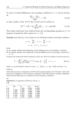
Table E4.5 presents a comparison of FDS of the explicit method with AS when central dif-
ferences are employed on the boundary conditions. Table E4.6 shows a similar comparison
when forward differences are employed on the boundary conditions.
(a)
Table E4.5. Comparison of FDS and AS at x =
0.30.

FDS AS Diff %Error
+->
0.00 1 1.0026 -0.0026 -0.0026
0.01 0.9984 0.9984 0.0001 0.0001
0.05 0.9475 0.9467 0.0008 0.0008
0.10 0.8719 0.8713 0.0006 0.0007
0.50 0.4401 0.4403 -0.0002 -0.0005
1.00 0.1871 0.1875 -0.0004 -0.0021