Page 116 - Computational Fluid Dynamics for Engineers

102 4. Numerical Methods for Model Parabolic and Elliptic Equations

T 2 1 sini2n+1)TO (E4A1)
= £ E rtvTv^ " ^
n=0
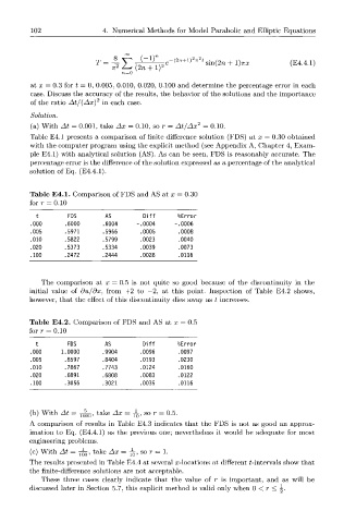
at x = 0.3 for t — 0, 0.005, 0.010, 0.020, 0.100 and determine the percentage error in each
case. Discuss the accuracy of the results, the behavior of the solutions and the importance
of the ratio At /(Ax) 2 in each case.
Solution.
(a) With At = 0.001, take Ax = 0.10, so r = At/Ax 2 = 0.10.
Table E4.1 presents a comparison of finite difference solution (FDS) at x = 0.30 obtained
with the computer program using the explicit method (see Appendix A, Chapter 4, Exam-
ple E4.1) with analytical solution (AS). As can be seen, FDS is reasonably accurate. The
percentage error is the difference of the solution expressed as a percentage of the analytical
solution of Eq. (E4.4.1).

Table E4.1. Comparison of FDS and AS at x = 0.30
for r = 0.10
FDS AS Diff %Error
+->
.000 .6000 .6004 -.0004 -.0006
.005 .5971 .5966 .0005 .0008
.010 .5822 .5799 .0023 .0040
.020 .5373 .5334 .0039 .0073
.100 .2472 .2444 .0028 .0116

The comparison at x = 0.5 is not quite so good because of the discontinuity in the
initial value of du/dx, from +2 to —2, at this point. Inspection of Table E4.2 shows,
however, that the effect of this discontinuity dies away as t increases.

Table E4.2. Comparison of FDS and AS at x = 0.5
for r = 0.10
t FDS AS Diff %Error
.000 1.0000 .9904 .0096 .0097
.005 .8597 .8404 .0193 .0230
.010 .7867 .7743 .0124 .0160
.020 .6891 .6808 .0083 .0122
.100 .3056 .3021 .0035 .0116

(b) With At = Y^Q, take Ax = ±, so r = 0.5.
A comparison of results in Table E4.3 indicates that the FDS is not as good an approx-
imation to Eq. (E4.4.1) as the previous one; nevertheless it would be adequate for most
engineering problems.
(c) With At = Y5Q, take Ax = ^ , s o r = l .
The results presented in Table E4.4 at several x-locations at different ^-intervals show that
the finite-difference solutions are not acceptable.
These three cases clearly indicate that the value of r is important, and as will be
discussed later in Section 5.7, this explicit method is valid only when 0 < r < \.