Page 113 - Computational Fluid Dynamics for Engineers

4.3 Discretization of Derivatives with Finite Differences 99

11 AX

t n+l
At
t n

t n-l

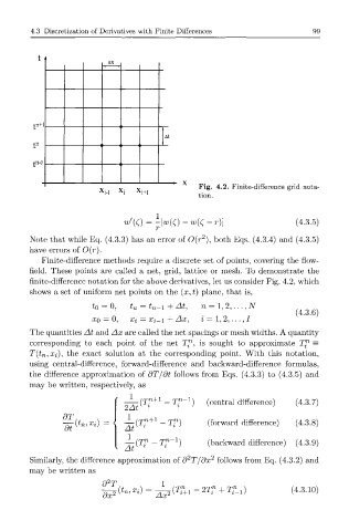
Fig. 4.2. Finite-difference grid nota-
M-l M+l tion.

/ 1
(C) = -KC)-^(C-r)] (4.3.5)
2
Note that while Eq. (4.3.3) has an error of 0(r ), both Eqs. (4.3.4) and (4.3.5)
have errors of 0(r).
Finite-difference methods require a discrete set of points, covering the flow-
field. These points are called a net, grid, lattice or mesh. To demonstrate the
finite-difference notation for the above derivatives, let us consider Fig. 4.2, which
shows a set of uniform net points on the (x, t) plane, that is,

2
to = 0, t n = t n-i + At, n = 1, , . . . , N
(4.3.6)
2
xo = 0, Xi = Xi-i + Ax, i = 1, , . . . , /
The quantities At and Ax are called the net spacings or mesh widths. A quantity
corresponding to each point of the net T™, is sought to approximate T/ 1 =
T(t n,Xi), the exact solution at the corresponding point. With this notation,
using central-difference, forward-difference and backward-difference formulas,
the difference approximation of dT/dt follows from Eqs. (4.3.3) to (4.3.5) and
may be written, respectively, as
{Tn +l nn—1\ (central difference) (4.3.7)
2At
(forward difference) (4.3.8)
AV * * '
( i f - i ; in—1> (backward difference) (4.3.9)
At
2
Similarly, the difference approximation of d T/dx 2 follows from Eq. (4.3.2) and
may be written as
2
d T n n
2 {tr, 2 (T t +1-2T t + T?_ (4.3.10)
dx Ax