Page 115 - Computational Fluid Dynamics for Engineers

4.4 Finite-Difference Methods for Parabolic Equations 101

i^ +1 T l = a A^( i +i- i + i -i (4.4.3a)
2T l T l
T l
i )
or
At
Tn +l^ Tn + a__ {Tn +i_ 2Tn + Tn_ i)j ; = 1 ; , . . . , J - 1 (4.4.3b)
2
From Eq. (4.4.3b) it is seen that, by this explicit formulation, the value of
n+
T 2 is expressed in terms of previous time values that are known, and the
2
equation allows the value of T to be obtained for i = 1, , . . . , I — 1. The values
of T at i = 0 and / are known from the boundary conditions. The numerical
error inherent in this scheme can be shown to be of order At + Ax 2 and, as a
result, the time step At must be kept small to ensure acceptable accuracy. In
addition, although explicit formulations are computationally simple, they can
lead to numerical instabilities unless the time step is also small. As is shown in
Section 5.7, in order to avoid the growth of errors in the operations for solving
Eq. (4.4.3), ^ must be < 1/2.

Example 4.1. Solve Eq. (4.2.4) subject to the following boundary and initial conditions

x = 0, T = 0; x = l , T = 0
2x 0 < x < k
t = 0 T =
2(1 -x) \<x<\
by the above explicit method for values of t = 0.005, 0.01, 0.02, 0.10 with a — 1 for three
different spacings in t,
5
—
a
( ^ = Tooo< ( b ) ^=iooo' ( c) At= 100
V ;
Compare your solutions with the analytical solution

At

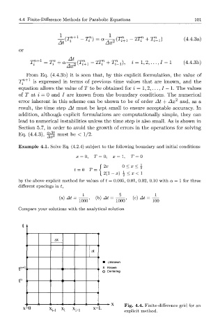
• Unknown
t n+1 X Known
O Centering
n
t

- x Fig. 4.4. Finite-difference grid for an
x=0 x x=L
M-l i 4+1 explicit method.