Page 117 - Computational Fluid Dynamics for Engineers

4.4 Finite-Difference Methods for Parabolic Equations 103

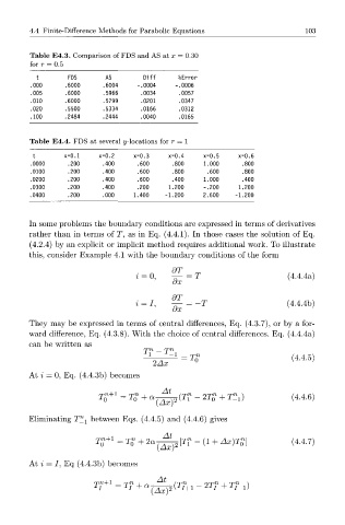
Table E4.3. Comparison of FDS and AS at x = 0.30
for r = 0.5
t FDS AS Diff %Error
.000 .6000 .6004 -.0004 -.0006
.005 .6000 .5966 .0034 .0057
.010 .6000 .5799 .0201 .0347
.020 .5500 .5334 .0166 .0312
.100 .2484 .2444 .0040 .0165

Table E 4 . 4 . FDS at several ^/-locations for r = 1
x=0.1 x=0.2 x=0.3 x=0.4 x=0.5 x=0.6
+->
.0000 .200 .400 .600 .800 1.000 .800
.0100 .200 .400 .600 .800 .600 .800
.0200 .200 .400 .600 .400 1.000 .400
.0300 .200 .400 .200 1.200 -.200 1.200
.0400 .200 .000 1.400 -1.200 2.600 -1.200

In some problems the boundary conditions are expressed in terms of derivatives
rather than in terms of T, as in Eq. (4.4.1). In those cases the solution of Eq.
(4.2.4) by an explicit or implicit method requires additional work. To illustrate
this, consider Example 4.1 with the boundary conditions of the form
dT
i = 0, — = T (4.4.4a)
ox

i = I, 9 £ = -T (4.4.4b)

They may be expressed in terms of central differences, Eq. (4.3.7), or by a for-
ward difference, Eq. (4.3.8). With the choice of central differences. Eq. (4.4.4a)
can be written as
rpn rpn
n
T 0 (4.4.5)
2Ax
At i — 0, Eq. (4.4.3b) becomes

n+1 n
T 0 = T 0 + aj^(Tf - 2T 0" + 7 ^ ) (4.4.6)
[ZAX)
Eliminating T ^ between Eqs. (4.4.5) and (4.4.6) gives

r n + i = n + 2a-^[T? - (1 + Ax)TZ\ (4.4.7)
T
At i = , Eq (4.4.3b) becomes
/
1
T^ = Tf + a ^ a (27+1 - 23? + 7?-i)