Page 114 - Computational Fluid Dynamics for Engineers

100 4. Numerical Methods for Model Parabolic and Elliptic Equations

4.4 Finite-Difference Methods for Parabolic Equations

The model equation used here to illustrate numerical methods for solving
parabolic partial-differential equations is the one-dimensional unsteady heat
conduction equation given by Eq. (4.2.4), which also serves as a model equation
for the boundary-layer equations, to be discussed in detail in Chapter 7.
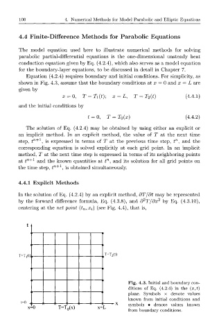
Equation (4.2.4) requires boundary and initial conditions. For simplicity, as
shown in Fig. 4.3, assume that the boundary conditions at x — 0 and x — L are
given by
x = 0, T = Ti(t); x = L, T = T 2(t) (4.4.1)
and the initial conditions by

t = 0, T = T 0(x) (4.4.2)

The solution of Eq. (4.2.4) may be obtained by using either an explicit or
an implicit method. In an explicit method, the value of T at the next time
n
step, £ n + 1 , is expressed in terms of T at the previous time step, t , and the
corresponding equation is solved explicitly at each grid point. In an implicit
method, T at the next time step is expressed in terms of its neighboring points
n + 1 n
at £ and the known quantities at t ', and its solution for all grid points on
n + 1
the time step, £ , is obtained simultaneously.
4.4.1 Explicit Methods

In the solution of Eq. (4.2.4) by an explicit method, dT/dt may be represented
2
by the forward difference formula, Eq. (4.3.8), and d T/dx 2 by Eq. (4.3.10),
centering at the net point (t n,Xi) (see Fig. 4.4), that is,

T=T 2 (t)
T=T 1(t) (

Fig. 4.3. Initial and boundary con-
ditions of Eq. (4.2.4) in the (x,t)
plane. Symbols x denote values
known from initial conditions and
t=0 1 symbols • denote values known
x=0 T=T 0(x) x=L
from boundary conditions.