Page 119 - Computational Fluid Dynamics for Engineers

4.4 Finite-Difference Methods for Parabolic Equations 105

(b)
Table E4.6. Comparison of FDS and AS at x =
0.30.
t FDS AS Diff %Error
0.00 1 1.0026 -0.0026 -0.0026
0.01 0.996 0.9984 -0.0024 -0.0024
0.05 0.9287 0.9467 -0.018 -0.019
0.10 0.8458 0.8713 -0.0255 -0.0292
0.50 0.403 0.4403 -0.0374 -0.0848
0.80 0.2313 0.2638 -0.0326 -0.1235
1.00 0.1597 0.1875 -0.0278 -0.1483

4.4.2 Implicit Methods: Crank—Nicolson

In contrast, implicit methods are unconditionally stable and allow significantly
larger time steps, with corresponding economy, as long as accuracy is main-
tained. For a parabolic partial differential, two popular implicit finite-difference
methods are due to Crank-Nicolson [1] and Keller [2]. Keller's method is dis-
cussed in subsection 4.4.3 for Eq. (4.2.4) and later in Chapters 7 and 8 for
boundary-layer and stability equations.
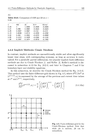
In this subsection, we describe the Crank-Nicolson method for Eq. (4.2.4).
2
This method uses the finite-difference grid shown in Fig. 4.5, where d T/dx 2 at
n+l 2
(t ' ,Xi) is expressed by the average of the previous and current time values
at t n and £ n + 1 , respectively,
n+1
2
O T .71+1/2 I +
dx 2 (*' Xi = — dx 2 dx 2 (4.4.10a)

• Unknown
t n+1 O X Known
Centering
At
t n

Fig. 4.5. Finite-difference grid for the
Crank-Nicolson method. Note that
while Ax is uniform, At can be
x=0 X i-1 M+l x=L nonuniform.