Page 112 - Computational Fluid Dynamics for Engineers

98 4. Numerical Methods for Model Parabolic and Elliptic Equations

4.3 Discretization of Derivatives with Finite Differences

Before the finite-difference methods for parabolic, hyperbolic and elliptic equa-
tions are described, it is useful to discuss the discretization of derivatives (either
ordinary or partial) with finite differences. For this purpose, consider a function
w which is single-valued, finite and continuous functions of £. Using Taylor's
theorem and with primes denoting differentiation with respect to C, we can write

2
w(( + r)= w(() + rw'(Q + \r w"(Q + ^ r V " ( C ) + • • • (4.3.1a)
and

2
3
w(C - r) = u;(C) - rw'(C) + \r w"{Q - \r v/"{Q + ••• (4.3.1b)
Adding both equations,
w(( + r) + w(C - r) = 2w(() + r V ( C )

provided the fourth- and higher-order terms are neglected. Thus,

W»(Q = -1 [w(( + r) - 2w(C) + w(C ~ r)] (4.3.2)

2
2
with an error of order r , 0(r ).
If Eq. (4.3.1b) is subtracted from Eq. (4.3.1a),
™'(C) = ^ K C + r ) - w ( C - r ) ] (4.3.3)

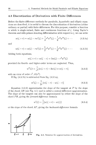
Equation (4.2.3) approximates the slope of the tangent at P by the slope
of the chord AB (see Fig. 4.1) and is called a central-difference approximation.
The slope of the tangent can also be approximated by either the slope of the
chord PJ5, giving the forward-difference formula

w'(C) = l[w(C + r)-w(0} (4.3.4)

or the slope of the chord AP, giving the backward-difference formula

\J\

Fig. 4.1. Notation for approximation of derivatives.