Page 132 - Computational Fluid Dynamics for Engineers

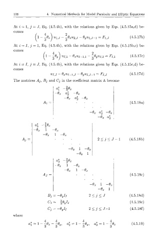
118 4. Numerical Methods for Model Parabolic and Elliptic Equations

At i — 1, j — J, Eq. (4.5.4b), with the relations given by Eqs. (4.5.15a,d) be-
comes
/ A 0x \ U 9
f 1 - ^ ) ^J ~ 3 ^ 2 , J - O yu\,j-i = Fi^j
(4.5.17b)
/
At i = , j = 1, Eq. (4.5.4b), with the relations given by Eqs. (4.5.15b,c) be-
comes
6y
1
7 2
3
V ~ i ) U1,1 ~~ 6xUl -^ 1 ~~ ^ ^ ' = Fl ^ (4.5.17c)
At i = , j = J, Eq. (4.5.4b), with the relations given by Eqs. (4.5.15c,d) be-
/
comes
UI,J - 8 XUI-\,J - OyU^j-i = F ItJ (4.5.17d)
The matrices Aj, Bj and Cj in the coefficient matrix A become

"-1 2> Ux
-u x &2 "x
a
~0 X 2
A,= (4.5.18a)
a%
j x tx 2 —6 X
a\
-6 X
a 3 px
3
1 -Ox
Ox 1
2 < j < J - 1 (4.5.18b)

1 -Ox
-Ox 1

1 -0 X
-Ox 1
Ar = (4.5.18c)

1 -6

B -Oyll 2 < j < J (4.5.18d)
3
d - -3Oyll (4.5.18e)

C 2 < j < J - l (4.5.18f)
j = -Oyh
where
4 4 4 4
(4.5.19)
3<