Page 155 - Computational Fluid Dynamics for Engineers

142 5. Numerical Methods for Model Hyperbolic Equations

A = (5.1.5a)
dQ
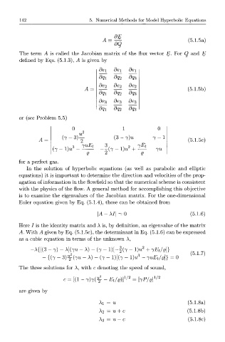
The term A is called the Jacobian matrix of the flux vector E. For Q and E
defined by Eqs. (5.1.3), A is given by

dei dei dei
dqi dq 2 dqs
de2 de2 de2
A = (5.1.5b)
dqi dq 2 dqs
des des des
dqi dq 2 dqs
3m 5.5)

0 1 0
u 2
(3 - j)u 7 - 1
A = ( 7 " 3 ) y (5.1.5c)
uE
/ i\ S l t JU
(7 - l)u - o ( 7 - l ) ^ + - —
p
z
Q
for a perfect gas.
In the solution of hyperbolic equations (as well as parabolic and elliptic
equations) it is important to determine the direction and velocities of the prop-
agation of information in the flowfield so that the numerical scheme is consistent
with the physics of the flow. A general method for accomplishing this objective
is to examine the eigenvalues of the Jacobian matrix. For the one-dimensional
Euler equation given by Eq. (5.1.4), these can be obtained from

\A-\I\ =0 (5.1.6)
Here I is the identity matrix and A is, by definition, an eigenvalue of the matrix
A. With A given by Eq. (5.1.5c), the determinant in Eq. (5.1.6) can be expressed
as a cubic equation in terms of the unknown A,
-A{[(3- 7 )-A](7«-A)-(7- 1)[ 3 ( 7 - V + 7^/2]}
(5.1.7)
- {(7 - 3)£( 7 « - A) - ( 7 - 1)[(7 " I K - -yuEt/g]} = 0

The three solutions for A, with c denoting the speed of sound,
1 / 2 1/2
c = [ ( i - 7 ) 7 ( ^ - ^ / e ) ] = [7P/e]
are given by

Ai = u (5.1.8a)
A2 = u + c (5.1.8b)
A3 = u — c (5.1.8c)