Page 158 - Computational Fluid Dynamics for Engineers

5.1 Introduction 145

and using the chain rule, we can write Eq. (5.1.4)

dQ dt dQ dx
or
*£•"£-• (5.1.18)

Multiplying both sides of Eq. (5.1.18) with X l and using Eq. (5.1.15), we
obtain
f-f- (5.1.19)

which is similar to Eq. (5.1.1) with hree uncoupled, independent equations.
t
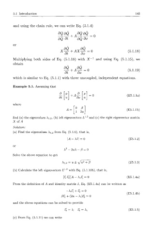
Example 5.1. Assuming that

d_ d
+ A 0 (E5.1.1a)
dt dx
where
0 P
A = (E5.1.1b)
1 2u
find (a) the eigenvalues Ai,2, (b) left eigenvectors L 1,2 and (c) the right eigenvector matrix
X of A
Solution:
(a) Find the eigenvalues Ai,2 from Eq. (5.1.6), that is,
\A-\I\ =0 (E5.1.2)

2
A - 2u\ - 0 = 0
Solve the above equation to get

= u± \/u 2 +(3 (E5.1.3)
Ai >2
1 2
(b) Calculate the left eigenvectors L ' with Eq. (5.1.10b), that is,
[i\r 2][A-xj} = o (E5.1.4a)
From the definition of A and identity matrix , Eq. (E5.1.4a) can be written as
/
-\il\ + l\ = 0
(E5.1.4b)
Pl\ + (2u - \i)li = 0
and the above equations can be solved to provide
l[ = i; li = \ z (E5.1.5)

(c) From Eq. (5.1.11) we can write