Page 162 - Computational Fluid Dynamics for Engineers

5.4 Implicit Methods 149

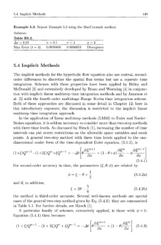
Example 5.3. Repeat Example 5.2 using the MacCormack method.
Solution:
Table E5.2.
Ax = 0.01 a = 0.1 <7 = 1 a = 2
=
Max Error (t --4) 0.0995605 0.0000018 Divergence

5.4 Implicit Methods

The implicit methods for the hyperbolic flow equation also use central, second-
order differences to discretize the spatial flux terms but use a separate time
integration. Schemes with these properties have been applied by Briley and
McDonald [3] and extensively developed by Beam and Warming [4] in conjunc-
tion with implicit linear multistep time integration methods and by Jameson et
al. [5] with the fourth-order multistage Runge-Kutta time integration scheme.
Both of these approaches are discussed in some detail in Chapter 12; here in
this introductory exposure, the discussion is restricted to the implicit linear
multistep time integration approach.
In the application of linear multistep methods (LMM) to Euler and Navier-
Stokes equations, it is seldom necessary to consider more than two-step methods
with three time levels. As discussed by Hirsch [1], increasing the number of time
intervals can put severe restrictions on the allowable space variables and mesh
points. A general two-step method with three time levels applied to the one-
dimensional scalar form of the time-dependent Euler equation, (5.1.2), is
ggn+1 Q En Q En-l
n
(l+£)Q n+1 -(l+20Q +£Q n_1 = ~At + (l-0 + (/>) '
dx dx dx
(5.4.1)
For second-order accuracy in time, the parameters (£, #, 0) are related by

4> = £-d+^ (5.4.2a)

and if, in addition,
£ = 28 - | (5.4.2b)
the method is third-order accurate. Several well-known methods are special
cases of the general two-step method given by Eq. (5.4.1): they are summarized
in Table 5.1. For further details, see Hirsch [1].
A particular family of schemes, extensively applied, is those with 0 = 0.
Equation (5.4.1) then becomes

0
(i + Q n + 1 - (i + 20Q n + ZQ"' 1 = -At ^ + < - c (5.4.3)