Page 163 - Computational Fluid Dynamics for Engineers

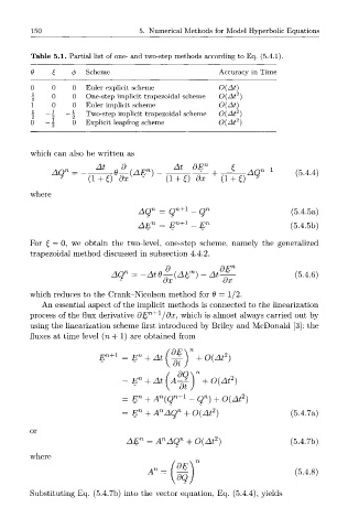
150 5. Numerical Methods for Model Hyperbolic Equations

Table 5.1. Partial list of one- and two-step methods according to Eq. (5.4.1)

0 £ (\> Scheme Accuracy in Time
0 0 0 Euler explicit scheme O(At)
2
\ 0 0 One-step implicit trapezoidal scheme 0(At )
1 0 0 Euler implicit scheme O(Ai)
2
| — \ — | Two-step implicit trapezoidal scheme 0(At )
2
0 — \ 0 Explicit leapfrog scheme 0(At )

which can also be written as

where

AQ n = Q n + 1 - Q n (5.4.5a)
n l
AE n = E + - E n (5.4.5b)
For £ = 0, we obtain the two-level, one-step scheme, namely the generalized
trapezoidal method discussed in subsection 4.4.2.
n n
AQ = -At6-^(AE ) - A t ^ - (5.4.6)
ox ox
which reduces to the Crank-Nicolson method for 9 = 1/2.
An essential aspect of the implicit methods is connected to the linearization
n+1
process of the flux derivative dE /dx, which is almost always carried out by
using the linearization scheme first introduced by Briley and McDonald [3]: the
fluxes at time level (n + 1) are obtained from

2
^ 1 +0(At )
d n
Q\ . „ , A l 2 ,

2
n
n
= E n + A (Q n+1 - Q ) + 0(At )
2
n
= E n + A AQ n + 0(At ) (5.4.7a)
or
n n n 2
AE = A AQ + 0(At ) (5.4.7b)
where 548
*"= I <- »

Substituting Eq. (5.4.7b) into the vector equation, Eq. (5.4.4), yields