Page 161 - Computational Fluid Dynamics for Engineers

148 5. Numerical Methods for Model Hyperbolic Equations

and determine the percentage error. Use second-order extrapolation on the numerical
boundary condition
ui = 2u?_! - < _ 2 (E5.2.3)
at x = 5.
Solution:
The computer program for this problem is given in Appendix A. Table E5.1 allows a
comparison of the numerical and analytical solutions (Max Error) as a function of Courant
number a. As discussed in Section 5.7, Eq. (5.7.20), stability requires a < 1.
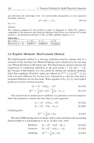
Table E5.1.
Ax = 0.01 (7 = 0.1 ( 7 = 1 (7 = 2
Max Error (t = 4) 0.0995775 0.0002478 Divergence

5.3 Explicit Methods: MacCormack Method

The MacCormack method is a two-step predictor-corrector scheme that is a
variation of the two-step Lax-Wendroff scheme and is identical to the one-step
Lax-Wendroff scheme in the linear case. The MacCormack method removes the
requirement of computing unknowns at the grid points i + 1/2 and i — 1/2,
and because of this feature, it is very useful for solving the nonlinear unsteady
Euler flow equations. Predictor values are defined at (t n+1 ,Xi) by u™ +1 (= ui)
with a forward difference for the flux term, followed by a corrector step with a
backward difference for the flux term. When applied to Eq. (5.1.1), this explicit
predictor-corrector method becomes

Ui = u? - a(u? +1 - uf) (5.3.1a)
< + 1 = \{u? + u?) ~\{u %- ui_ x) (5.3.1b)

This method can be written more explicitly in a predictor-corrector sequence
where the symmetry between the two steps is more apparent.
^ = uf - c r « + 1 - u?) (5.3.2a)
Ui = uf — a(ui — Ui-i) (5.3.2b)

Updating gives
< + 1 = ^ i + 5i) (5.3.2c)
The above differencing can be reversed, and in some problems such as moving
discontinuities it is advantageous to do so. In that case, write
Predictor Ui = uf - a(uf - i^-i) (5.3.3a)
Corrector Ui — u™ — cr(ui+i — u~i) (5.3.3b)

Updating u^ 1 = ~{Ui + ui) (5.3.3c)