Page 165 - Computational Fluid Dynamics for Engineers

152 5. Numerical Methods for Model Hyperbolic Equations

Solution:
First rewrite Burger's equation (4.2.8) in vector form similar to Eq. (5.1.2),

and then substitute
2
E = u /2, A = u (E5.4.3)
in Eq. (5.4.8). The finite difference approximation to this equation is given by Eq. (5.4.9)
which is applicable for all i except at the outflow boundary, i = J, at which we represent
^- with backward differencing and write

1
7
A n , Atu^Au } -vJj^Au }^ At tT?KAA\
AUl + = (El El l] ( E 5 A 4 )
A~x 2 ~A^ ~ -
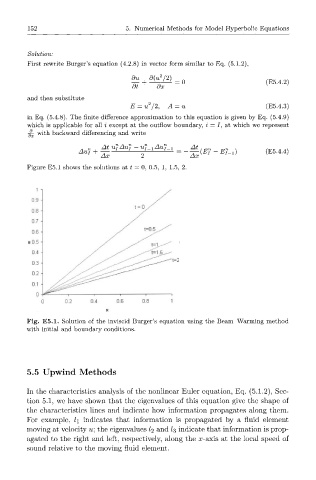
Figure E5.1 shows the solutions at t = 0, 0.5, 1, 1.5, 2.

Fig. E5.1. Solution of the inviscid Burger's equation using the Beam-Warming method
with initial and boundary conditions.

5.5 Upwind Methods

In the characteristics analysis of the nonlinear Euler equation, Eq. (5.1.2), Sec-
tion 5.1, we have shown that the eigenvalues of this equation give the shape of
the characteristics lines and indicate how information propagates along them.
For example, l\ indicates that information is propagated by a fluid element
moving at velocity u] the eigenvalues I2 and Z3 indicate that information is prop-
agated to the right and left, respectively, along the x-axis at the local speed of
sound relative to the moving fluid element.