Page 167 - Computational Fluid Dynamics for Engineers

154 5. Numerical Methods for Model Hyperbolic Equations

solution of nonlinear equations and multi-dimensional problems with upwind
methods.
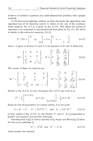
In the flux-vector-splitting method, we first determine the eigenvalues and
eigenfunctions of the Jacobian matrix A, which, in the case of the nonlinear
Euler equation, Eq. (5.1.2), is given by Eq. (5.1.5). This allows the system of
equations to be expressed in one-dimensional form given by Eq. (5.1.19) which
is similar to the convective equation, (5.1.1).
Ai
l
X~ AX = A = u-\- c (5.5.7)
A 3 u — c
where c is given in Section 5.1 and X is the product of M and TV defined by
- Q Q
1 0 0 y/2c V2c
- 1
1
M Q 0 N = 71 71 (5.5.8)
u 1
QU QC QC
L~2 7 - 1 ,
V2 V2
The inverse of these two matrices are

1 0 0 0
1
0 1 1
1
1
M' = T V " - (5.5.9)
Q y/2 y/2gc
- 1 1
( 7 - l ) y ( ! - 7 ) « 7 - 1
7 2 \/2QCJ
Similar to Eq. (5.5.2), we next decompose Eq. (5.5.7) and write it as
1 [ A i ± | A i |
A± = 2 (^±1^1) (5.5.10)
= »\ A 2 ±|A 2 |
I A 3 ±|A 3 |

Based on this decomposition, we express matrix A in two parts
1
A = A + + A~, A + = XA+X' , and A~ = XA~X~ l (5.5.11)
so that, similar to Eq. (5.5.2), we can identify A + and A~ as corresponding to
positive and negative characteristic directions.
Assuming that E(Q) is a linear function of Q, Steger and Warming [5] define
the flux-vector-splitting by
+
E + = A Q and E~ = A~Q (5.5.12)
which satisfies the relations