Page 172 - Computational Fluid Dynamics for Engineers

5.6 Finite-Volume Methods 159

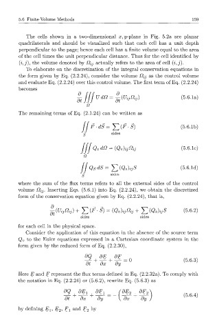
The cells shown in a two-dimensional #, y-plane in Fig. 5.2a are planar
quadrilaterals and should be visualized such that each cell has a unit depth
perpendicular to the page; hence each cell has a finite volume equal to the area
of the cell times the unit perpendicular distance. Thus for the cell identified by
(i, ), the volume denoted by ftij actually refers to the area of cell (i,j).
j
To elaborate on the discretization of the integral conservation equations in
the form given by Eq. (2.2.24), consider the volume ftij as the control volume
and evaluate Eq. (2.2.24) over this control volume. The first term of Eq. (2.2.24)
becomes
^ tjjjudQ = ^ t{U ijQ lJ) (5.6.1a)
Q
The remaining terms of Eq. (2.1.24) can be written as

d S = ^ ( F - S ) (5.6.1b)
/ /
sides

JJJ Q v dQ = {Q v)ijQij (5.6.1c)
n

II Q sdS=J2(Qsh s ( - - )
5 6 ld
g sides
where the sum of the flux terms refers to all the external sides of the control
volume fiij. Inserting Eqs. (5.6.1) into Eq. (2.2.24), we obtain the discretized
form of the conservation equation given by Eq. (2.2.24), that is,

5 6 2
^Uijiiii) +J2(F-§) = [Q v)ijQij + Y, (Q*h S ( - - )
sides sides
for each cell in the physical space.
Consider the application of this equation in the absence of the source term
to the Euler equations expressed in a Cartesian coordinate system in the
Q v
form given by the reduced form of Eq. (2.2.30),
dQ dE OF ,

Here E and F represent the flux terms defined in Eq. (2.2.32a). To comply with
the notation in Eq. (2.2.24) or (5.6.2), rewrite Eq. (5.6.3) as

d
A + ?Ml + ^ 1 _ (?1k + ?Il) (5.6.4)
=
dt dx dy \ dx dy J
by defining E x, E 2, F x and F 2 by