Page 176 - Computational Fluid Dynamics for Engineers

5.6 Finite-Volume Methods 163

u
m 1/2 i i-H 1/2
1 i - N
• J • • 9 • I
— - Q i — ^
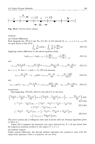
Fig. E5.2. Grid for finite volume.

Solution:
(a) Central differences
First integrate Eq. (E5.5.1) [see Eq. (2.1.24)] in the interval Qi, Xi_i/ 2 < x < Xi+1/2, for
the grid shown in Fig. E5.2.
f 4-(v4)dx= f 4-("^r)<te (E5.5.3)
JQ d% J Q. dx \ ax J

Applying central differences to the above equation yields,

(«*) <+i/2 - W>);-i/2 = (y^-) - (v^-) (E5.5.4)
and
0Z+1 + 4>i </>i + fa-l <t>i+\ — <t>i </>i ~ <f>i-l / — r r\
^t+i/2 2 u i-i/2 g = ^ + 1 / 2 2 ^ ^ ~ 1 / 2 A r (E5.5.5)
for 1 < i < N. For i = 1 and i = N, (E5.5.4) becomes
02 + 01 , , nx 02 - 01 01 - 0(0) . .
wi + 1/2 2 ^1-1/20(0) = ^ 1 + 1 / 2 — ^ ^1-1/2 A x / 2 (E5.5.6)
and
i/ r x 0N +07V-1 0(L) - 0JV 07V-0/V-1 , „ _ - -v
^iV+l/20W - UN-1/2 ~ = ^7V + l/2 ~A~~f^ "N-l/2 "7 (E5.5.7)
respectively.
Rearrange Eqs. (E5.5.6), (E5.5.5) and (E5.5.7) in the form

(u 1+1/2 1/1+1/2 . 2 i / i _ i / 2 \ /W1+1/2 ^1+1/2 \ , / . 2 z / 1 _ i / 2 \ 0(0)
(,-2- + "ST + ~Ax-) ^ + \—2 Ax-) ^ = [ Ul -^ 2 + -Ax-)
(E5.5.8a)
( Uj-l/2 ^-1/ 2 \ / • /^ i + 1/2 ^ - 1 / 2 • "i+1/2 • ^-1/ 2 \ ,
(E5.5.8b)

, v . ' (E5.5.8c)
= ( - ^ + 1 / 2 + ^ m / i ) ( A ( L )
The above system has a tridiagonal form and is solved with the Thomas algorithm given
in Table 4.1.
Figure E5.3 compares the numerical and exact solutions for N = 10 and shows that
the numerical solutions oscillate in the region 0.7 < x < 1.
(b) Upwind method
Unlike central differences, the upwind method represents the convective term with the
values from upstream. Since u is positive, we can write