Page 173 - Computational Fluid Dynamics for Engineers

160 5. Numerical Methods for Model Hyperbolic Equations

y
A

(U+i)
Ci (B

h (i-lj) (U) (i+lj)
\
D A
(Ml)

~+r-k—•

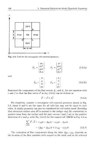
Fig. 5.3. Grid for the rectangular cell-centered geometry.

gu
9
Si = F T = 2 (5.6.5a)
gv z
E tu
E tv
and
0
V 0
£ (5.6.5b)
92 ^ 2
0
pv
Represent the components of the flux vectors E 1 and F l for one equation with
e and / so that the flux vector F in Eq. (5.6.2) can be written as

F = ei + fj (5.6.6)

For simplicity, consider a rectangular cell-centered geometry shown in Fig.
5.3, where k and h are the same for all cells but may not be equal to each
other. A similar geometry can also be considered for cell-vertex mesh. Recalling
that elemental surface area dS is normal to the surface and (by convention) is
positive away from the surface and the unit vectors i and j are in the positive
directions of x and y, write Eq. (5.6.2) for the control cell ABCD in Fig. 5.3 as

^2 F - S = e ABh + f Bck ~ ecD& - / D A ^
sides
= (/BC - /DA)& + (CAB - ecv)h (5.6.7)
e
The evaluation of flux components along the sides /BCO AB> depends on
the location of the flow variables with respect to the mesh and on the selected