Page 177 - Computational Fluid Dynamics for Engineers

164 5. Numerical Methods for Model Hyperbolic Equations

(W0i+l/2 = U i + i/ 2<t>i, {u(j)) i_ 1/2 = Ui-i/ 2<l>i-l (E5.5.9)

and Eq. (E5.5.4) is represented by
J. JL (pi+1 - <t>i <j>i ~ (pi-1 / - o r tr i n \
Ui+i/iQi - Ui-i/ 2(t>i-i = ^i+1/2 ~r ^i-1/2 ~r (E5.5.10)

At nodes 1 and TV, Eq. (E5.5.4) becomes

Wi + l/201 - ^1-1/20(0) = 1/1 + 1/2 ^ - ^1-1/2 ^ i (E5.5.11)

and

JL JL (f)(L) - (f) N </>7V - 4>N~1 /T^C r 1 0 \
UN + 1/2<PN - U N-i/ 2<pN-l = ^iV + 1/2 , /g "N-l/2 ~T (E5.5.12)
Express Eqs. (E5.5.10-12) in a tridiagonal form and solve

/ . ^ 1 + 1/2 ^ 1 - 1 / 2 \ , ^ 1 + 1/2 . / . ^ 1 - 1 / 2 \ , / n x / n r r i Q \

^«i +i/2 + " ^ - + ^ j J <A! - -^-<h = ^«i-i/2 + ^ - J 0(0) (E5.5.13a)
-
/ ^ - l / 2 \ , / ^i+1/2 . ^i-l/2 \ , ^i+1/2 , n / T ^ r - i o i N

/ VN-l/2\ , ( 2lS N + 1/2 1/^-1/2^ , 2^Ar + 1 / 2
(-tiAT-1/2 " " ^ J *N-1 + ( ^ - 1 / 2 + — 3 ^ - + — ^ J <t>N = —^-<KL)
(E5.5.13c)
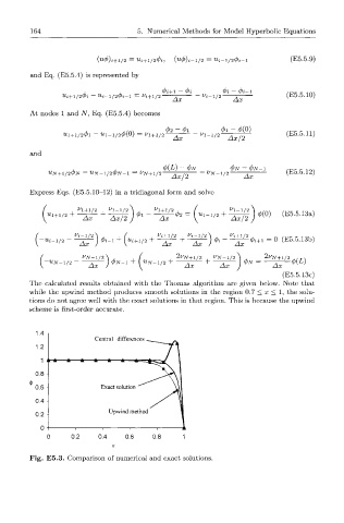
The calculated results obtained with t h e Thomas algorithm are given below. Note that
while the upwind method produces smooth solutions in th e region 0.7 < x < 1, th e solu-
tions do not agree well with the exact solutions in hat region. This is because th e upwind
t
scheme is first-order accurate.
1.4
Central differences
1.2
1
0.8
0.6 Exact solution

0.4
Upwind method
0.2 H
0
0 0.2 0.4 0.6 0.8
X
Fig. E 5 . 3 . Comparison of numerical an d exact solutions.