Page 195 - Computational Fluid Dynamics for Engineers

6.3 Finite-Difference Method 183

this case, the solution of the Laplace equation expressed in polar coordinates,
Eq. (P2.19.2), which can be written as

^ + 1 ^ + 1 ^ = 0 (6.3.1)
dr 2 r dr r 2 d6 2

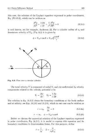
is well known, see for example, Anderson [2]. For a cylinder radius of r*o and
freestream velocity of V^ (Fig. 6.3) it is given by

cos#
= Foorcos^ + Kooro (6.3.2)

Fig. 6.3. Flow over a circular cylinder.

The total velocity V is composed of radial V r and circumferential VQ velocity
components related to the velocity potential 4> by

ldcf)
V r V e (6.3.3)
dr' r~d9
The solution in Eq. (6.3.2) obeys the boundary conditions at the body surface
and at infinity, see Eqs. (6.2.8) and (6.2.9), which in our case can be written as

r = r 0 , * 0 (6.3.4a)
or
oo, -+ Vr^rcosO (6.3.4b)
Before we discuss the numerical solution of the Laplace equation expressed
in polar coordinates, Eq. (6.3.1), it is useful to express this equation and its
boundary conditions in dimensionless forms. For this purpose, define