Page 197 - Computational Fluid Dynamics for Engineers

6.3 Finite-Difference Method 185

I
77
\
A D
1

B C
0 ^
0 n/2 n

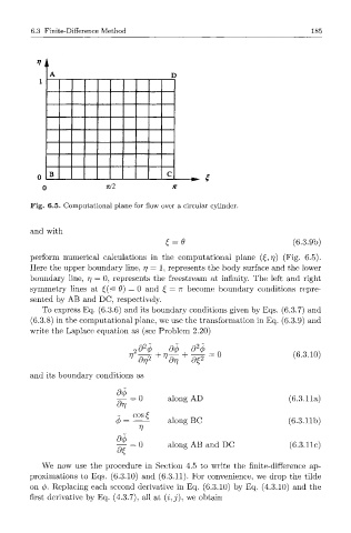
Fig. 6.5. Computational plane for flow over a circular cylinder.

and with
(6.3.9b)

perform numerical calculations in the computational plane (£, rj) (Fig. 6.5).
Here the upper boundary line, r\ = 1, represents the body surface and the lower
boundary line, r\ = 0, represents the freestream at infinity. The left and right
symmetry lines at £(= 6) = 0 and £ = TT become boundary conditions repre-
sented by AB and DC, respectively.
To express Eq. (6.3.6) and its boundary conditions given by Eqs. (6.3.7) and
(6.3.8) in the computational plane, we use the transformation in Eq. (6.3.9) and
write the Laplace equation as (see Problem 2.20)

d±
2&± + - 0 (6.3.10)
dr\ 2 drj + &e
and its boundary conditions as

along AD (6.3.11a)
Of]
c o s
1 £ along BC (6.3.11b)
0 =
V
I- along AB and DC (6.3.11c)

We now use the procedure in Section 4.5 to write the finite-difference ap-
proximations to Eqs. (6.3.10) and (6.3.11). For convenience, we drop the tilde
on (j). Replacing each second derivative in Eq. (6.3.10) by Eq. (4.3.10) and the
j
first derivative by Eq. (4.3.7), all at (i, ), we obtain