Page 202 - Computational Fluid Dynamics for Engineers

190 6. Inviscid Flow Equations for Incompressible Flows

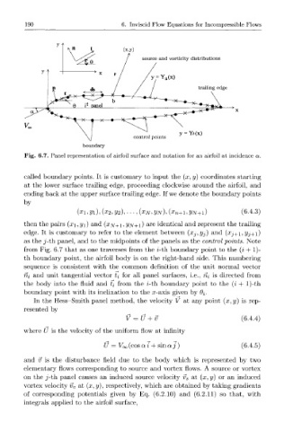
Fig. 6.7. Panel representation of airfoil surface and notation for an airfoil at incidence a.

called boundary points. It is customary to input the (x, y) coordinates starting
at the lower surface trailing edge, proceeding clockwise around the airfoil, and
ending back at the upper surface trailing edge. If we denote the boundary points
by
(xi, 2/1), (x 2,2/2), • • •, (x N, y N), (x n + i, 2/w+i) (6.4.3)

then the pairs (xi, y\) and (xyv+1, yN+i) a r e identical and represent the trailing
edge. It is customary to refer to the element between (xj,yj) and ( X J + I , ? / J + I )
as the -th panel, and to the midpoints of the panels as the control points. Note
j
from Fig. 6.7 that as one traverses from the i-th boundary point to the (i + 1)-
th boundary point, the airfoil body is on the right-hand side. This numbering
sequence is consistent with the common definition of the unit normal vector
Hi and unit tangential vector ti for all panel surfaces, i.e., Hi is directed from
the body into the fluid and U from the i-th boundary point to the (i + l)-th
boundary point with its inclination to the x-axis given by Q{.
In the Hess-Smith panel method, the velocity V at any point (x, y) is rep-
resented by
V = U + v (6.4.4)
where U is the velocity of the uniform flow at infinity

U = Voo(cosai + sin a j ) (6.4.5)

and v is the disturbance field due to the body which is represented by two
elementary flows corresponding to source and vortex flows. A source or vortex
on the -th panel causes an induced source velocity v s at (x, y) or an induced
j
vortex velocity v v at (x, y), respectively, which are obtained by taking gradients
of corresponding potentials given by Eq. (6.2.10) and (6.2.11) so that, with
integrals applied to the airfoil surface,