Page 200 - Computational Fluid Dynamics for Engineers

188 6. Inviscid Flow Equations for Incompressible Flows

Table 6.1. Numerical and analytical dimensionless velocity potential results

£ = --2° £ = = 90° £ = 178°
V rnum </>an rnum 0 a n Y^num 0 a n
0.12 8.38 8.45 0.00 0.00 -8.38 -8.45
0.2 5.16 5.20 0.00 0.00 -5.16 -5.20
0.3 3.61 3.63 0.00 0.00 -3.61 -3.63
0.4 2.88 2.90 0.00 0.00 -2.88 -2.90
0.5 2.48 2.50 0.00 0.00 -2.48 -2.50
0.6 2.25 2.26 0.00 0.00 -2.25 -2.26
0.7 2.12 2.13 0.00 0.00 -2.12 -2.13
0.8 2.04 2.05 0.00 0.00 -2.04 -2.05
0.9 2.00 2.01 0.00 0.00 -2.00 -2.01
0.98 1.99 2.00 0.00 0.00 -1.99 -2.00

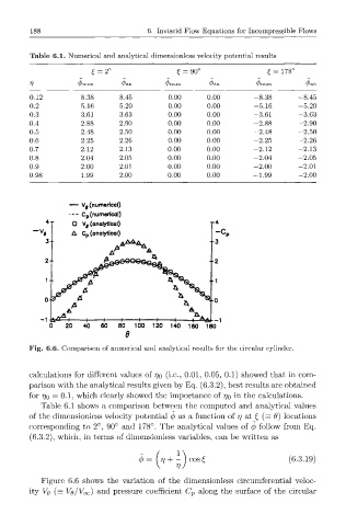
— Vj (numerical)
— C p (numerical)
O Vj (analytical)
A C p (analytical)

100 120 140 160 180

Fig. 6.6. Comparison of numerical and analytical results for the circular cylinder.

calculations for different values of 770 (i.e., 0.01, 0.05, 0.1) showed that in com-
parison with the analytical results given by Eq. (6.3.2), best results are obtained
for 770 = 0.1, which clearly showed the importance of 770 in the calculations.
Table 6.1 shows a comparison between the computed and analytical values
of the dimensionless velocity potential 0 as a function of 77 at £ (= 9) locations
corresponding to 2°, 90° and 178°. The analytical values of (f) follow from Eq.
(6.3.2), which, in terms of dimensionless variables, can be written as

77 H— I cos £ (6.3.19)

Figure 6.6 shows the variation of the dimensionless circumferential veloc-
ity VQ = VQ/VOQ) and pressure coefficient C p along the surface of the circular
(