Page 206 - Computational Fluid Dynamics for Engineers

194 6. Inviscid Flow Equations for Incompressible Flows

6.5 A Panel Program for Airfoils

In this section a computer program is described for calculating the inviscid flow-
field over an airfoil with the Hess-Smith panel method that was discussed in the
previous section (see also Appendix B). Before reviewing the four subroutines
and MAIN of this program, it is useful to examine the solution of Eqs. (6.4.13)
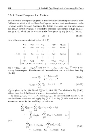
and (6.4.14), which can be written in the form given by Eq. (4.5.23), that is,

(4.5.23)

Here A is a square matrix of order (N + 1)
an au • .. aij . .. a 1N Gl,JV+l
a<2i ^22 • .. a 2j . .. a 2N «2,7V+1

A = an a>%2 • a^ any ttz,JV+l (6.5.1)

ayvi ayv2 ... ajsfj ... a^jy ajv,N+i
a
a
a
| N+l,l OJV+1,2 • • • N+lj • • • N+l,N Q>N+1,N+1
T T
and x = (qi,...,qi,-..,qN,T) and b= (6i,..., &*,..., b N, b N+i) with T de-
noting the transpose. The elements of the coefficient matrix A follow from Eq.
(6.4.14)
z = l,2,...,7V
— A n
n- a %3 — J\ %3, (6.5.2a)
j = l,2,...,7V
N
B
«i,N+i = Y, & < = l,2,...,iV (6.5.2b)
J = I
A% are given by Eq. (6.4.9) and B% by Eq. (6.4.11). The relation in Eq. (6.5.1)
follows from the definition of x where r is essentially £AT+I-
To find ajsr+ij (J = 1,..., N) and a7v+i,7V+i in the coefficient matrix A, we
use the Kutta condition and apply Eq. (6.4.13) to Eq. (6.4.8b) and, with r as
a constant, we write the resulting expression as
N N
T
v
B
(
Y^ AjQj + Yl h + °° cos a - °i)
3 = 1 3=1
N N
V
T
I Y At NjQj + Y1 B Nj + oo cos(a - 0 N)
13=1 3=1
or as
N N
£ ( 4 , + 4,)^- + r ](^ + B* )
J
Nj
(6.5.3)
3=1 3=1
= -Foo cos(a -Oi)-Voo cos(a - 6>^)