Page 236 - Computational Fluid Dynamics for Engineers

7.4 Computer Program BLP 225

VGP K is the variable-grid parameter. Use K = 1.0 for laminar flow and
K = 1.14 for turbulent flow. For a flow consisting of both laminar and
turbulent flows, use K = 1.14.
RL Reynolds number, ^oL.
Surface distance, feet or meters, or dimensionless.
Velocity, feet per second or meter per second, or dimensionless.
u e

7.4.3 Subroutine IVPL

At £ = 0, Eq. (7.3.6) reduces to the Falkner-Skan equation, Eq. (7.3.11), which
can be solved subject to the boundary conditions of Eq. (7.3.7). Since the equa-
tions are solved in linearized form, initial estimates of j , Uj and Vj are needed
/
in order to obtain the solutions of the nonlinear Falkner-Skan equation. Various
expressions can be used for this purpose. Since Newton's method is used, how-
ever, it is useful to provide as good an estimate as is possible and an expression
of the form.
3rjj 1 (i)} °
u (7.4.8)
i = ~
2 Ve
usually satisfies this requirement. The above equation is obtained by assuming
a third-order polynomial of the form

f = a + br) + erf

and by determining constants a, 6, c from the boundary conditions given by
Eq. (7.3.7) for the zero-mass transfer case and from one of the properties of
momentum equation which requires that f" — 0 at 77 = rj e.
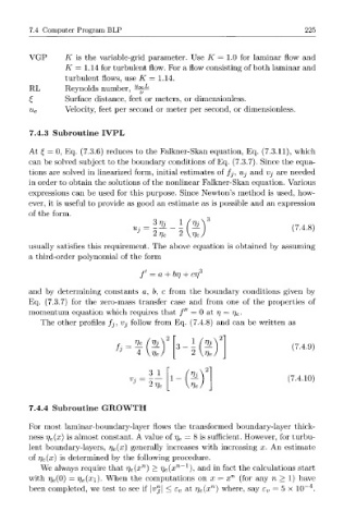
The other profiles / j , Vj follow from Eq. (7.4.8) and can be written as

_ rj e (ai) 2 3 -- 1 / 'V, .VI
h 4 UJ 2^ KVeJ (7.4.9)

3 1
Vj = 1 - (% )1 (7.4.10)
\Ve, /
2r] e
7.4.4 Subroutine G R O W T H

For most laminar-boundary-layer flows the transformed boundary-layer thick-
ness rj e(x) is almost constant. A value of rj e = 8 is sufficient. However, for turbu-
lent boundary-layers, rj e(x) generally increases with increasing x. An estimate
of r} e(x) is determined by the following procedure.
n l
n
We always require that rj e(x ) > rj e(x ~ ), and in fact the calculations start
with 7/ e(0) = rj e(xi). When the computations on x = x n (for any n > 1) have
n
- 4
|
been completed, we test to see if ^ j | < e v at r) e(x ) where, say e v = 5 x 10 .