Page 232 - Computational Fluid Dynamics for Engineers

7.3 Numerical Method for the Standard Problem 221

( So). - -/i-l&W +'^& ) - ^ f - 1 (7.3.25b)

^
(*3)i = f " ! » , + « 2 „,n-l (7.3.25c)
^ - 1 / 2
OL\ (y) a" „n-i
*4j 2-^A + T V i / 2 (7.3.25d)

(")
(S5)j = -a2MJ' (7.3.25e)

(s 6 )i = -a2Mj-i (7.3.25f)
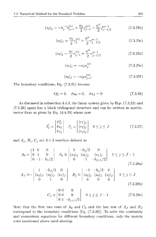
The boundary conditions, Eq. (7.3.21) become

Sfo = 0, 6UQ = 0, foxj = 0 (7.3.26)

As discussed in subsection 4.4.3, the linear system given by Eqs. (7.3.23) and
(7.3.26) again has a block tridiagonal structure and can be written in matrix-
vector form as given by Eq. (4.4.29) where now

Sfj (n)j
*i 8UJ f j = iT2)j 0 < j < J (7.3.27)
(rsh
6 Vj
and Aj, Bj, Cj are 3 x 3 matrices defined as

1 0 0 1 -hj/2 0
0 1 0 Ai = («3)j («5)j (Sl)j 1 < j < J - 1
0 - 1 -W2 0 - 1 -h j+1/2
(7.3.28a)
1 -hj/2 0 - 1 -hj/2 0

A A (S3)j (S5)j {Sl)j Bi (s 4 )j (s 6)j {s 2)j 1 < J < J
0 1 0 0 0 0
(7.3.28b)
0 0 0
Cj 0 0 0 0 < j < J - 1 (7.3.28c)
0 1 -/ij+i/2
Note that the first two rows of AQ and CQ and the last row of Aj and Bj
correspond to the boundary conditions [Eq. (7.3.26)]. To solve the continuity
and momentum equations for different boundary conditions, only the matrix
rows mentioned above need altering.