Page 235 - Computational Fluid Dynamics for Engineers

224 7. Boundary-Layer Equations

In most problems, calculations are performed by selecting hi and K and
calculating the transformed boundary-layer thickness r) e. An idea about the
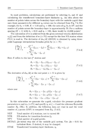
number of points taken across the boundary-layer with the variable 77-grid that
uses those parameters for different r] e-values can be obtained from Fig. 7.4. For
4
example, for h\ — 0.01, K = 1.10 and r\ e = 100, the ratio oir} e/h\ is 10 , and the
number of points across the boundary-layer is approximately 70. For a uniform
spacing (K = 1) with hi = 0.01 and rj e = 100, there would be 10,000 points!
The calculation of m is achieved from the given external velocity distribution
u e{C) and from the definition of m (= P2) except for the first NX-station where
P2(l) is read in. The derivative of du e/d^ (DUDS) is obtained by using three-
point Lagrange interpolation formulas given by (n < N):

2 n+ n l]
=
(1f) " \ {in+l ~ u) + % {u+l ~ ^ * -
B
vn+l (7.4.4)
+ ^ - ( £ n - £ n - l )
Here N refers to the last £ n station and

M = (£ n - fn-l)(fn+l ~ fn-l)
= (£n ~ £n-l)(£n+l - £n) (7-4.5)
A 2
-43 = (£n+l - £n)(£n+l ~ f n - l )
The derivative of du e/d^ at the end point n = TV is given by

du e\ u^~ 2 u^~ l
-77- = — 1 — ( € N ~ 6 v - i ) + - ^ — ( 6 v ~ &V-2)

where now
M = (€N-I - £N-2)(£,N ~ C7V-2)
= (£N-I - 6v- 2 )fcv ~ 6 v - i ) (7.4.7)
A 2
M = (£N - €N-I)(€N - €N-2)
In this subroutine we generate the 77-grid, calculate the pressure gradient
parameters m and m\ (= PI) and specify rj e at £ = 0 and the reference Reynolds
number R^ (RL). In addition, the following data are read in and the total
number of j-points J(NP) is computed from Eq. (7.4.3).

NXT Total number of ^-stations, not to exceed 60
NTR NX-station for transition location £tr
NPT Total number of 77-grid points.
DETA(l) Z\n-initial step size of the variable grid system. Use An — 0.01 for
turbulent flows. If desired, it may be changed.
ETAE Transformed boundary-layer thickness, rj e