Page 229 - Computational Fluid Dynamics for Engineers

218 7. Boundary-Layer Equations

7.3.1 Numerical Formulation

In order to express Eqs. (7.3.6) and (7.3.7) as a system of first-order equations,
we define new variables u(^rj) and v(^rj) by

f' = u (7.3.12a)

(7.3.12b)
and write Eqs. (7.3.6) and (7.3.7) as

ra + 1 „ ,„ _ / du df
/7 x/ 9x (7.3.12c)
m
(H + -y~f v + (* - u ) = £ ( ^ - ^
7^ = 0, iz = 0, f = f w(x); V = Ve, u = l (7.3.13)

We denote the net points of the net rectangle shown in Fig. 4.6, modified below
due to a slight change in notation, by

Co = 0, £n = f n_! + fc n, n = 1, , . . . , TV
2
(7.3.14)
7?0 = 0, 7ft =77 <7-_i + fy, j = l , 2 , . . . , J
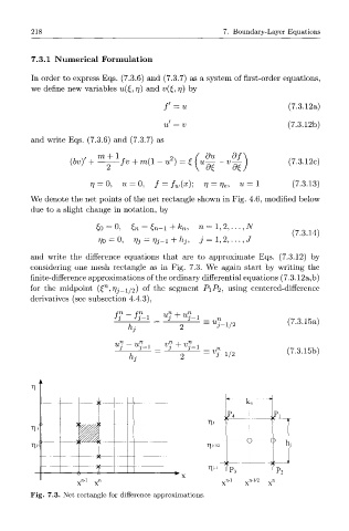
and write the difference equations that are to approximate Eqs. (7.3.12) by
considering one mesh rectangle as in Fig. 7.3. We again start by writing the
finite-difference approximations of the ordinary differential equations (7.3.12a,b)
n
for the midpoint (^ ,Tjj-1/2) °f the segment P1P27 using centered-difference
derivatives (see subsection 4.4.3),

ff-ff-l_,."? + tt?-l n
= 1 2 (7.3.15a)
h, ~ 2 ^ ' - /
«"-«"-! _ «" + «"_!
= t) (7.3.15b)
i-1/2

i L
^
7^
^ j£
t\*
^---f~
Tli-i T|J-i/2 hj
f
^ Ui-i "
n x „-l x n-,/2 x n
<""' X
Fig. 7.3. Net rectangle for difference approximations.