Page 226 - Computational Fluid Dynamics for Engineers

7.2 Standard, Inverse and Interaction Problems 215

negligible, the inviscid flow solutions can be improved by incorporating viscous
effects into the inviscid flow equations [4].
A convenient and popular approach is based on the concept that the dis-
placement surface can also be formed by distributing a blowing or suction ve-
locity on the body surface. The strength of the blowing or suction velocity v^ is
determined from the boundary-layer solutions according to

(7.2.6)
ax
where x is the surface distance of the body, and the variation of v\> on the body
surface simulates the viscous effects in the potential flow solution. This approach
can be used for both incompressible and compressible flows as discussed in [4].

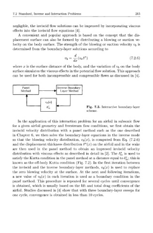
Panel Inverse Boundary-
^ Layer Method
Method r w
k k,
v x
b( )
^
1 K Fig. 7.2. Interactive boundary-layer
scheme.

In the application of this interaction problem for an airfoil in subsonic flow
for a given airfoil geometry and freestream flow conditions, we first obtain the
inviscid velocity distribution with a panel method such as the one described
in Chapter 6, we then solve the boundary-layer equations in the inverse mode
so that the blowing velocity distribution, v^x), is computed from Eq. (7.2.6)
and the displacement thickness distribution 8*(x) on the airfoil and in the wake
are then used in the panel method to obtain an improved inviscid velocity
distribution with viscous effects as described in detail in [2]. The 6% e is used to
satisfy the Kutta condition in the panel method at a distance equal to <$£,; this is
known as the off-body Kutta condition (Fig. 7.2). In the first iteration between
the inviscid and the inverse boundary-layer methods, vi{x) is used to replace
the zero blowing velocity at the surface. At the next and following iterations,
a new value of v^x) in each iteration is used as a boundary condition in the
panel method. This procedure is repeated for several cycles until convergence
is obtained, which is usually based on the lift and total drag coefficients of the
airfoil. Studies discussed in [4] show that with three boundary-layer sweeps for
one cycle, convergence is obtained in less than 10 cycles.