Page 287 - Computational Fluid Dynamics for Engineers

9.5 Differential Equation Methods 277

(a) (b)

(c) (d)
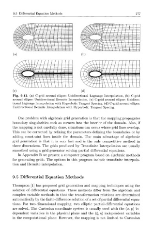
Fig. 9.12. (a) C-grid around ellipse: Unidirectional Lagrange Interpolation, (b) C-grid
around ellipse: Unidirectional Hermite Interpolation, (c) C-grid around ellipse: Unidirec-
tional Lagrange Interpolation with Hyperbolic Tangent Spacing, (d) C-grid around ellipse:
Unidirectional Hermite Interpolation with Hyperbolic Tangent Spacing.

One problem with algebraic grid generation is that the mapping propagates
boundary singularities such as corners into the interior of the domain. Also, if
the mapping is not carefully done, situations can occur where grid lines overlap.
This can be corrected by refining the parameters defining the boundaries or by
adding constraint lines inside the domain. The main advantage of algebraic
grid generation is that it is very fast and is the only competitive method in
three dimensions. The grids produced by Transfinite Interpolation are usually
smoothed using a grid generator solving partial differential equations.
In Appendix B we present a computer program based on algebraic methods
for generating grids. The options in this program include transfinite interpola-
tion and Hermite interpolation.

9.5 Differential Equation Methods

Thompson [1] has proposed grid generation and mapping techniques using the
solution of differential equations. These methods differ from the algebraic and
complex variable methods in that the transformation relations are determined
automatically by the finite-difference solution of a set of partial differential equa-
tions. For two-dimensional mapping, two elliptic partial-differential equations
are solved. The Cartesian coordinate system is usually used with the (x,y) in-
dependent variables in the physical plane and the (£, rj) independent variables
in the computational plane. However, the mapping is not limited to Cartesian