Page 286 - Computational Fluid Dynamics for Engineers

276 9. Grid Generation

^ - J / L ^ i
\ P.P. /
V
/ N
/ X / ! \
i' N v
: ^—
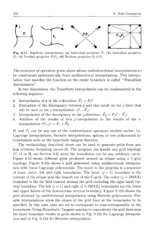
Fig. 9.11. Algebraic interpolation; (a) Individual projector Pi; (b) Individual projector
Pj\ (c) Product projector PiPj\ (d) Boolean projector Pi 0 Pj.

The structure of operators given above allows multidirectional interpolations to
be constructed systematically from unidirectional interpolations. This interpo-
lation that matches the function on the entire boundary is called "Transfinite
Interpolation".
In two dimensions, the Transfinite Interpolation can be implemented in the
following sequence:
1. Interpolation of r in the i-direction: F\ = Pi?
2. Evaluation of the discrepancy between r and this result on the j-lines that
will be used in the j-interpolation: (? — F\)
3. Interpolation of the discrepancy in the j-direction: F2 — Pj?— F\)
4. Addition of the results of this ^'-interpolation to the results of the i-
interpolation: ?(i,j) = F\ + F2
Pi and Pj can be any one of the unidirectional operators studied earlier, i.e.
Lagrange interpolations, Hermite interpolations, splines, or non-polynomial in-
terpolations such as the hyperbolic tangent function.
The methodology described above can be used to generate grids from any
four arbitrary bounding curves [4]. The program can handle any grid topology
(C, O or H, see Section 9.6) since the boundaries can be any arbitrary curve.
Figure 9.12 shows different grids produced around an ellipse using a C-grid
topology. Figure 9.12a shows a grid generated using unidirectional interpola-
tion with linear Lagrange polynomials. The input to the program is a sequence
of inner, outer, left and right boundaries. The inner (j = 1) boundary is the
contour of the ellipse plus the branch cut of the C-grid. The outer {j = JMAX)
boundary is the far field contour around the grid excluding the right hand ver-
tical boundary. The left (i = 1) and right (i — IMAX) boundaries are the lower
and upper halves of the downstream vertical boundary. Figure 9.12b shows the
grid obtained by unidirectional interpolation using Hermite polynomials. Her-
mite interpolations allow the slopes of the grid lines at the boundaries to be
specified. In this case, they are set to correspond to near-orthogonality at the
boundaries. Using Hyperbolic Tangent spacing to concentrate the grid lines near
the inner boundary results in grids shown in Fig. 9.12c for Lagrange interpola-
tion and in Fig. 9.12d for Hermite interpolation.