Page 281 - Computational Fluid Dynamics for Engineers

9.4 Algebraic Methods 271

The upper and lower boundaries may be written as

(9.4.9)
XB2 = X 2(0 = f, VB2 = V2(0 = 1 + £
This produces the mapping required in Eq. (9.4.7) and is of the form

x = £ (9.4.10a)

3/=(1 + 0*7 (9.4.10b)
The metrics of this transformation for the continuity equation (9.3.4) are

9 4 n
& = i , z = o, Vx = - ^ , »fo = T ^ < - - )
v

9.4.1 Algebraic Grid Generation Using Transfinite Interpolation

To generate algebraic grids around more complex configurations, a multi-
directional interpolation method called "Transfinite Interpolation" is often used.
This method is implemented as a suite of unidirectional interpolations.

Unidirectional Interpolation

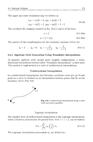
In a unidirectional interpolation, the Cartesian coordinate vector r(x, y) of each
point on a curve is obtained as an interpolation between points that lie on the
boundary curves (Fig. 9.8).

Fig. 9.8. Unidirectional interpolation along a curve
=
ii 0 with end points specified.

Lagrange Interpolation
The simplest form of unidirectional interpolation is the Lagrange interpolation,
which is based on polynomials. Its general form, with 1 < i < , can be written:
/

7 1 = 1 ^ '
The Lagrange interpolation polynomials (j) n are defined by: