Page 279 - Computational Fluid Dynamics for Engineers

9.4 Algebraic Methods 269

the centerline by AB and the upper surface by DC, with the ordinate of the
nozzle upper surface given by

y 1 < x < 2 (9.4.1)
It is clear that for this geometry a rectangular grid in the physical plane is not
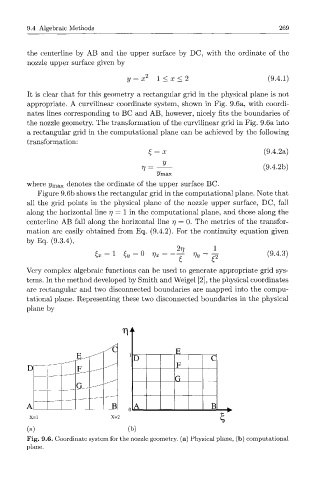
appropriate. A curvilinear coordinate system, shown in Fig. 9.6a, with coordi-
nates lines corresponding to BC and AB, however, nicely fits the boundaries of
the nozzle geometry. The transformation of the curvilinear grid in Fig. 9.6a into
a rectangular grid in the computational plane can be achieved by the following
transformation:
f = x (9.4.2a)
r] = -^— (9.4.2b)
2/max
where 2/ max denotes the ordinate of the upper surface BC.
Figure 9.6b shows the rectangular grid in the computational plane. Note that
all the grid points in the physical plane of the nozzle upper surface, DC, fall
along the horizontal line rj = 1 in the computational plane, and those along the
centerline AB fall along the horizontal line rj = 0. The metrics of the transfor-
mation are easily obtained from Eq. (9.4.2). For the continuity equation given
by Eq. (9.3.4),

6* = 1 Zy = Q Vx = ~j V y = ^ (9.4.3)
Very complex algebraic functions can be used to generate appropriate grid sys-
tems. In the method developed by Smith and Weigel [2], the physical coordinates
are rectangular and two disconnected boundaries are mapped into the compu-
tational plane. Representing these two disconnected boundaries in the physical
plane by

k

^£ R
I
D C
F
D[ F _
G
G _

A B A B
0
X=2
%
(a) (b)
Fig. 9.6. Coordinate system for the nozzle geometry, (a) Physical plane, (b) computational
plane.