Page 274 - Computational Fluid Dynamics for Engineers

264 9. Grid Generation

of the transformation and knowing the one-to-one correspondence of the loca-
tion of each grid point in both computational and physical planes in order to
transform the solution back to the physical plane.
In the brief discussion of grid generation methods presented in this chapter,
the basic concepts of the mapping and development of curvilinear coordinates
are discussed in Section 9.2. Descriptions of three grid generation techniques,
starting with the simplest scheme in one dimension (Section 9.3) are given In
Sections 9.4 to 9.6. Section 9.7 will briefly review basic concepts and techniques
for generating unstructured grids.

9.2 Basic Concepts in Grid Generation and Mapping

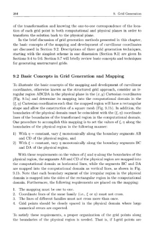
To illustrate the basic concepts of the mapping and development of curvilinear
coordinates, otherwise known as the structured grid approach, consider an ir-
regular region ABCDA in the physical plane in the (x, y) Cartesian coordinates
(Fig. 9.1a) and determine its mapping into the computational domain in the
(£, rj) Cartesian coordinates such that the mapped region will have a rectangular
shape and allow the construction of a square mesh (Fig. 9.1b). In addition, the
boundaries of the physical domain must be coincident with the (£, rj) coordinate
lines of the boundaries of the transformed region in the computational domain.
One procedure to accomplish this mapping is to set the values of £, rj along the
boundaries of the physical region in the following manner:

1) With 77 = constant, vary £ monotonically along the boundary segments AB
and CD of the physical region, and
2) With £ = constant, vary rj monotonically along the boundary segments BC
and DA of the physical region.
With these requirements on the values of £ and rj along the boundaries of the
physical region, the segments AB and CD of the physical region are mapped into
the computational domain as horizontal lines, while the segments BC and DA
are mapped into the computational domain as vertical lines, as shown in Fig.
9.1b. Note that each boundary segment of the irregular region in the physical
domain is mapped into the sides of the rectangular region in the computational
domain. Furthermore, the following requirements are placed on the mapping:

1. The mapping must be one to one.
2. Coordinate lines of the same family (i.e., £ or rj) must not cross.
3. The lines of different families must not cross more than once.
4. Grid points should be closely spaced in the physical domain where large
numerical errors are expected.

To satisfy these requirements, a proper organization of the grid points along
the boundaries of the physical region is needed. That is, if I-grid points are